Analysis Methods

Once you load or create a network in SocNetV, you may use the options in the Analyze menu to compute graph and social network analysis measures.

Tip

Analysis on filtered subgraphs: When graph exploration filters are active (ego network, focus on selection, filter by attribute, filter by centrality, or edge weight filter), all computations — matrices, cohesion measures, centrality, community detection — operate only on the currently visible nodes and edges. Hidden nodes are excluded from calculations. This lets you analyze a specific subgraph without modifying the underlying data.

---

Matrix Analysis

Options to compute, display, and analyze various matrices based on the adjacency matrix of the current network.

Adjacency Matrix

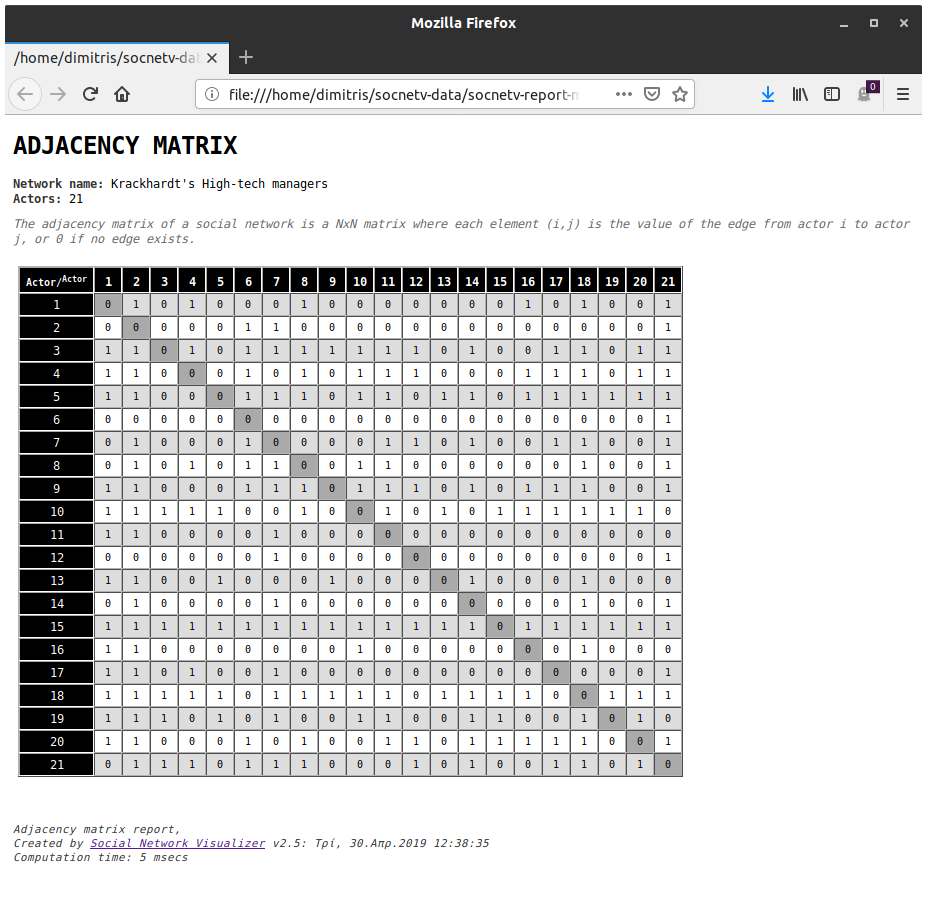
Displays the adjacency matrix $A$ of the active network. The matrix is displayed in HTML format in your default web browser.

The adjacency matrix of a social network is a matrix where each element $a(i,j)$ is equal to the weight of the arc from actor (node) $i$ to actor $j$. If the actors are not connected, then $a(i,j) = 0$.

---

Inverse Adjacency

This option computes the inverse $A^{-1}$ of the adjacency matrix.

---

Plot Adjacency

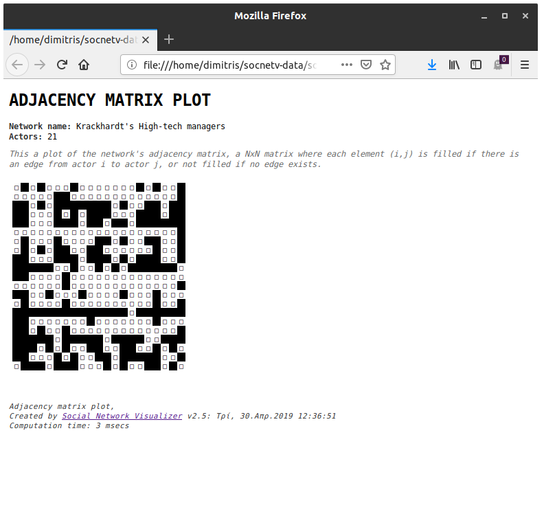
To plot the adjacency matrix, you can also press Shift+F6. The plot will appear in your web browser.

---

Transpose Adjacency

This option computes the transpose of the adjacency matrix.

---

Cocitation Matrix

Computes the Cocitation matrix, $C = A^T \cdot A$.

The matrix $C$ is an $n \times n$ symmetric matrix where each element $c(i,j)$ is the number of actors that have outbound ties/links to both actors $i$ and $j$. The diagonal elements $c_{ii}$ of the Cocitation matrix are equal to the number of inbound edges of $i$ (inDegree).

---

Degree Matrix

This option computes the Degree matrix of the network. The Degree Matrix is a diagonal matrix that contains information about the degree of each graph vertex (row of the adjacency matrix).

---

Laplacian Matrix

This option computes the Laplacian matrix of the network. The Laplacian is an $N \times N$ matrix $L = D - A$, where $D$ is the degree matrix of $A$.

---

Cohesion Measures

The next option in the Analyze menu focuses on basic network/graph measures, such as the geodesic distance between nodes, the mean distance between all nodes, the diameter of the graph, the number of geodesics between nodes, and the eccentricity of each node. Each option is explained below.

Note

The Density of the graph/network is computed automatically and you can always see it on the right sidebar (Statistics Panel > Network)

---

Reciprocity

Reciprocity, $r$, is a measure of the likelihood of vertices in a directed network to be mutually linked.

SocNetV supports two different methods to index the degree of reciprocity in a social network:

• Arc reciprocity: The fraction of reciprocated ties over all actual ties in the network.

• Dyad reciprocity: The fraction of actor pairs that have reciprocated ties over all pairs of actors that have any connection.

In a directed network, the arc reciprocity measures the proportion of directed edges that are bidirectional. If the reciprocity is 1, then the adjacency matrix is structurally symmetric.

Likewise, in a directed network, the dyad reciprocity measures the proportion of connected actor dyads that have bidirectional ties between them.

In an undirected graph, all edges are reciprocal. Thus the reciprocity of the graph is always 1.

Reciprocity can be computed on undirected, directed, and weighted graphs.

Concretely, if $L$ is the total number of ties (arcs) in the network and $L_{\leftrightarrow}$ is the number of those ties that are reciprocated (i.e. the reverse arc also exists), then:

$$r_{arc} = \frac{L_{\leftrightarrow}}{L}$$

Similarly, if $M$ is the number of actor pairs that have at least one tie between them, and $M_{\leftrightarrow}$ is the number of those pairs with ties in both directions, then:

$$r_{dyad} = \frac{M_{\leftrightarrow}}{M}$$

---

Symmetry Test

The Symmetry Test reports whether the network is symmetric or not. A network is called “symmetric” if for every edge $(i,j)$ in the set $E$ of the corresponding graph $G(V,E)$, the opposite $(j,i)$ edge also exists in $E$. In other words, when the adjacency matrix is symmetric.

---

Distance

Computes the geodesic distance (length of the shortest path) between two actors, and shows you the exact sequence of intermediate nodes along that path.

In graph theory, the shortest path between two vertices of the graph is called a geodesic.

Thus, the geodesic distance of two nodes in a social network is the length of the shortest path between the corresponding vertices in the graph $G(V,E)$.

By clicking on the Analyze → Cohesion → Distance option (or pressing Ctrl+G, Ctrl+G), you will be asked to pick a source and a target node. SocNetV then displays:

• The geodesic distance — the number of hops (edges) on the shortest path.
• The shortest path itself — the ordered sequence of nodes from source to target, using node labels where available (e.g. Alice → Carol → Bob).

For unweighted networks SocNetV uses Breadth-First Search (BFS), which guarantees the shortest hop-count path in O(V + E) time.
For weighted networks SocNetV uses Dijkstra’s algorithm, which finds the minimum-cost path in O((V + E) log V) time.

Tip

The edges along the reported path are also selected on the canvas, exactly as if you had Shift-clicked each one in turn. This lets you immediately move, inspect, or right-click the whole path without hunting for it visually — useful on large or dense networks where the path is hard to trace by eye. Only the path’s edges are selected, not its nodes, so the highlight doesn’t pull in unrelated edges attached to those same nodes.

---

Average Distance

The average or mean distance in a social network is the average length of all shortest paths (geodesics) between all pairs of connected vertices in the corresponding graph.

In undirected or strongly connected directed networks, the formula used to compute Average Graph Distance is:

$$\bar{d} = \frac{\sum_{u \neq v}{d(u,v)}}{n \cdot (n-1)}$$

where the denominator is the sum of all pairs of vertices.

It can be proved that in connected networks of $n$ actors, the least upper bound of the Average Distance is $\frac{n+1}{3}$ (Doyle & Graver, 1977).

In the case of disconnected networks/graphs, the denominator used is the total number of existing paths between connected vertices.

In graph theory, the Average Distance is considered to be a natural measure of the compactness of a graph.

---

Geodesic Distance Distribution

The Analyze → Cohesion → Geodesic Distance Distribution option (shortcut Ctrl+G, Ctrl+I) answers the question: how many pairs of nodes are exactly d hops apart?

For each distance value $d = 1, 2, \ldots, D$ (where $D$ is the diameter of the network), SocNetV counts the number of ordered connected pairs separated by exactly that distance and produces a report table:

Distance (d)	Pairs	% of connected pairs	Cumulative %
1	…	…	…
2	…	…	…
…	…	…	…

Unreachable pairs (nodes in different weakly connected components) are excluded from the count.

What the distribution reveals:

• Small-world networks typically show most pairs clustered at distance 2–3, with a rapid cumulative rise and a low diameter relative to network size.
• Sparse or chain-like networks show a flat, spread-out distribution with pairs at many different distances.
• The average distance $\bar{d}$ is the weighted mean of this distribution: $\bar{d} = \sum_d d \cdot P(d)$, where $P(d)$ is the fraction of pairs at distance $d$.

The computation re-uses the all-pairs shortest-path (APSP) cache produced by any prior distance or centrality calculation, so it is fast when the cache is warm.

---

Distances Matrix

The Analyze -> Cohesion -> Distances Matrix menu option displays the matrix of geodesic distances between all pairs of nodes in the social network.

A distances matrix is an $N \times N$ square matrix, in which the $(i,j)$ element is the distance from node $i$ to node $j$.

---

Geodesics Matrix

This option displays an $n \times n$ square matrix, where the $(i,j)$ element is the number of geodesics between node $i$ and node $j$. The produced matrix, called the sigma matrix, is used in Centralities calculation (see below).

---

Eccentricity

The eccentricity or association number of each node $u$ is the largest geodesic distance between that node and every other node in the network.

$$\epsilon_u = \max{\{d(u,v), \forall v \in V\}}$$

Therefore, the measure reflects how far, at most, each node is from every other node.

The Eccentricity can be calculated in both graphs and digraphs but is usually best suited for undirected graphs.

It can also be calculated in weighted graphs: real edge weights are used as shortest-path costs (or their inverse, if you choose to invert weights) — see Edge Weights above for guidance.

Note

This raw eccentricity $\epsilon_u$ is a distance, not a centrality score — larger means less central. See Eccentricity Centrality (EC) below for the standardized, inverted version ($EC_u = 1/\epsilon_u$) used to rank nodes by centrality.

---

Diameter

The diameter of a social network is the maximum eccentricity of any vertex in the corresponding graph $G(V,E)$, that is, the maximum distance between any two connected nodes.

$$D = \max{\{d(u,v), \forall u,v \in V\}}$$

---

Connectedness

In plain terms: can you get from any actor to any other actor by following ties, possibly through intermediaries? Connectedness answers exactly that, and reports how many separate “islands” (components) the network splits into if the answer is no.

In an undirected graph, this is unambiguous: a graph is connected if there is a path between every pair of nodes, and disconnected otherwise, with the report telling you how many disconnected components exist.

In a directed graph, edge direction creates two genuinely different, both meaningful, notions of “connected” — so SocNetV asks you which one you mean before computing:

• Weak connectivity — treats every edge as if it were bidirectional, i.e. ignores arrow direction entirely. This answers “how many disconnected islands are there, if I don’t care which way information can flow?” A directed chain $A \to B \to C$ is weakly connected even though there’s no way back from $C$ to $A$.
• Strong connectivity — respects edge direction. The network is strongly connected only if every node can both reach, and be reached from, every other node via directed paths. The same chain $A \to B \to C$ is not strongly connected, since $C$ cannot reach $A$.

Formally:

• A digraph is strongly connected if, for every pair of nodes $(i,j)$, there is a directed path from $i$ to $j$ and a directed path from $j$ to $i$.
• A digraph is weakly connected if every pair of nodes is joined by a semipath — a path in the underlying undirected graph, ignoring direction.

Strong connectivity is always the stricter condition: any strongly connected digraph is automatically weakly connected too, but not the reverse. So a directed network can be reported “weakly connected” while still failing the strong test — if that happens, run Connectedness again and choose Strong to see the directed-reachability picture instead.

A graph or digraph is disconnected if it has more than one component (in the undirected case) or more than one weakly-connected component (in the directed case) — in particular, any isolated node on its own makes the network disconnected.

Tip

Use Layout → Node Color by Connected Component to visualize the separate components directly on the canvas when a network turns out to be disconnected.

---

Node Connectivity

Node Connectivity asks a very concrete question about two specific actors: if an adversary (or a random failure) could remove other nodes from the network, how many would they need to remove to cut off actor A from actor B? A low number means that pair’s connection depends on just a few “bridge” actors — a structural vulnerability; a high number means many independent routes exist between them.

Formally, for two non-adjacent nodes $s$ and $t$, the local vertex connectivity $\kappa(s,t)$ is the minimum number of nodes — other than $s$ and $t$ themselves — whose removal disconnects $t$ from $s$.

By Menger’s theorem (Menger, 1927), this minimum “cut” size is always exactly equal to the maximum number of internally vertex-disjoint paths between $s$ and $t$ — paths that share no intermediate node. So $\kappa(s,t)$ simultaneously answers “how many nodes must fail to disconnect them?” and “how many completely independent routes exist between them?” — the two are the same number. SocNetV computes it via a maximum-flow algorithm on an internal representation of the network built specifically for this purpose (each node split into an “in” and “out” half joined by a capacity-1 link), which is the standard way to turn Menger’s theorem into an efficient computation.

If $s$ and $t$ are directly tied, node connectivity is not defined — the edge between them is a “path” that no removal of other nodes can ever break, so SocNetV reports “directly connected” rather than a number.

By Analyze → Cohesion → Node Connectivity, you pick a source and a target node. On a directed network, you’re also asked whether to respect edge direction:

• Weak: treats every edge as bidirectional.
• Strong: counts only the nodes needed to block directed paths from source to target — note that $\kappa(s,t)$ and $\kappa(t,s)$ can differ under this mode, since blocking the forward direction doesn’t necessarily block the reverse one.

---

Graph Connectivity

Graph Connectivity asks the same question as Node Connectivity, but network-wide: what is the fewest nodes that would need to be removed to disconnect the network at its single weakest point?

Formally, the global vertex connectivity $\kappa(G)$ is the minimum of $\kappa(s,t)$ over every non-adjacent pair of nodes $(s,t)$ in the network — i.e. the worst-case (most vulnerable) pair anywhere in the graph.

$\kappa(G)$ is a standard measure of a network’s robustness to targeted or random node failure: a low $\kappa(G)$ (e.g. 1, an actual “cut vertex” whose removal splits the network) flags a single point of failure, while a high $\kappa(G)$ means the network keeps functioning even after several actors are removed.

A useful sanity bound (Whitney’s inequality, Whitney 1932) is that $\kappa(G)$ can never exceed $\delta(G)$, the minimum degree in the network — you can always disconnect the least-connected node from the rest just by removing all of its neighbors. SocNetV uses this bound to skip unnecessary computation where possible.

By Analyze → Cohesion → Graph Connectivity, on a directed network you are likewise asked to choose Weak or Strong (matching the same choice offered by Connectedness and Node Connectivity above).

---

Walks of a Given Length

Clicking this option asks for a desired walk length (max: $n-1$). Then SocNetV calculates and displays a square matrix where each element $(i,j)$ is the number of walks of the given length between the corresponding pair of nodes $i$ and $j$.

A walk is a sequence of alternating vertices and edges such as:

$$v_0e_1, v_1e_2, v_2e_3, \dots, e_kv_k$$

where each edge, $e_i$, is defined as $e_i = \{v_{i-1}, v_i\}$.

This function calculates the number of walks of the given length between each pair of nodes, by studying the powers of the sociomatrix.

---

Total Walks

Calculates and displays an $n \times n$ square matrix whose elements denote the number of walks of any length between each pair of nodes. The algorithm is based on the powers of the sociomatrix.

Warning: This function is VERY SLOW on large networks ($n > 50$), since it will calculate all powers of the sociomatrix up to $n-1$ in order to find out all possible walks. If you need to make a simple reachability test, we advise you to use the Reachability Matrix function instead.

---

Reachability Matrix

Calculates the reachability matrix $X^R$ of the graph where each $(i,j)$ element is 1 if nodes $i$ and $j$ are reachable, otherwise 0.

This function is based on the Distances Matrix; it checks whether the corresponding element of the Distances matrix is not zero. If it is not zero, then the nodes $(i,j)$ are reachable, and the $X^R$ element is 1.

---

Clustering Coefficient

In graph theory, a clustering coefficient reflects the degree to which the nodes tend to cluster together. In social network analysis, it is often used to characterize the transitivity of a network.

There are two versions of the Clustering Coefficient: the global and the local.

The global Clustering Coefficient (often called transitivity, see Wasserman and Faust, 1994, page 243) is based on triplets of nodes to give an indication of the overall clustering in the whole network.

A triplet consists of three connected nodes. A triangle, therefore, includes three closed triplets, one centered on each of the nodes.

The global clustering coefficient is the number of closed triplets (or 3 x triangles) over the total number of triplets (both open and closed). This metric can be applied to both undirected and directed networks.

The local Clustering Coefficient (introduced by Duncan J. Watts and Steven Strogatz in 1998) is an indication of the embeddedness of single nodes, and it is also used as an indication of the network transitivity.

Specifically, the Clustering Coefficient $C$ of a node quantifies how close the node and its neighbors are to being a complete subgraph (clique).

Let $k_i$ be the number of vertices, $|N_i|$, in the neighborhood, $N_i$, of a node $i$.

In a directed network, the clustering coefficient is computed with the formula:

$$C_i = \frac{|\{e_{jk}: v_j,v_k \in N_i, e_{jk} \in E\}|}{k_i(k_i-1)}$$

In undirected networks, the formula is:

$$C_i = \frac{2|\{e_{jk}: v_j,v_k \in N_i, e_{jk} \in E\}|}{k_i(k_i-1)}$$

If the network relation represents friendships among actors, the clustering coefficient $C_i$ of an actor $i$ measures the ratio of existing friendships between any two of that actor’s friends relative to all possible friendships between her friends (the situation where the subgraph is complete).

A value close to one indicates that the node is involved in many transitive relations.

SocNetV also computes the network average clustering coefficient (Watts and Strogatz):

$$\bar{C} = \frac{1}{n} \sum_{i=1}^{n} C_i$$

Note: The clustering can be used to determine whether a network is a small-world or not.

Tip

The local Clustering Coefficient is also available as a node color gradient layout: go to Layout → Node Color → Clustering Coefficient (shortcut Ctrl+L, Ctrl+C, Ctrl+G) to color nodes from blue (low CLC) to red (high CLC). See Node Color by Clustering Coefficient in the Visualization page.

For the ring lattice, the clustering coefficient is:

$$C(0) = \frac{3(K-2)}{4(K-1)}$$

tending to $\frac{3}{4}$ as $K$ grows, where $K$ is the mean degree.

---

All the basic network statistics, such as nodes, edges and density are displayed and automatically updated in the Analysis tab of the left dock in SocNetV main window.

---

Centralities and Prestige

The last option in the Analysis menu opens the “Centrality and Prestige” sub-menu.

In social network analysis (SNA), researchers use various measures to assess the prominence or importance of each node (actor) within a network. These measures help identify influential individuals or key entities in the network. For example, in a social network, we might want measure the importance of a person based on the number of friends they have, or we could want to identify a person who is highly respected by others in the network. In another example, we might want to know how critical a power station is inside the power company grid…

Although there are various metrics for calculating node importance, they are generally classified into two broad categories: Centrality and Prestige. These concepts are foundational in social network analysis, drawing on the work of Wasserman and Faust (1994), as well as Knoke and Burt (2001), who distinguish between centrality as a measure of connectivity and prestige as a measure of status or recognition within a network.

Centrality

Centrality measures quantify the relative importance of a node based on its position within the network. Central nodes are typically well-connected, either through direct connections or by bridging gaps between other nodes.

SocNetV supports a wide variety of centrality indices, including those conceptualized by Wasserman and Faust, such as:

• Degree Centrality (DC): Measures the number of direct connections a node has. A node with high degree centrality is considered well-connected within the network.

• Closeness Centrality (CC): Measures how close a node is to all other nodes, based on the length of the shortest paths. A node with high closeness centrality can reach other nodes quickly.

• Betweenness Centrality (BC): Measures how often a node lies on the shortest path between two other nodes. Nodes with high betweenness centrality have significant control over information flow within the network.

• Eigenvector Centrality (EVC): Measures the influence of a node by considering both the number of connections it has and the importance of the nodes it is connected to. A node connected to other high-scoring nodes will have a higher score.

• Eccentricity Centrality (EC): Measures the longest shortest path from a node to all other nodes in the network. The node with the lowest eccentricity is considered the most “central” in terms of distance.

• Influence Range Closeness Centrality (IRCC): A variation of Closeness Centrality that considers only the nodes reachable from a given node, making it useful for disconnected networks.

• Stress Centrality (SC): Measures how often a node appears on the shortest paths between other nodes. High stress centrality indicates a node is a key intermediary or bridge within the network.

• Power Centrality (PC): A generalized degree centrality (Gil-Schmidt) that credits a node for its whole neighborhood at every distance, weighted so closer neighbors count for more.

• Information Centrality (IC): Uses all paths between actors, not just the shortest ones, weighted by tie strength and distance.

• Katz Centrality (KC) and Bonacich Power Centrality (BPC): give a node credit for indirect connections (friends-of-friends, and so on), discounted the further away they are — useful when Eigenvector Centrality’s own decay collapses to zero on sparse or directed networks.

These centrality measures focus on the node’s direct connections, its geodesic distances, or its ability to influence others through its position in the network. Wasserman and Faust’s conceptualization of centrality focuses on connectivity and control, with a particular emphasis on how nodes serve as intermediaries or closers in the network.

Prestige

In contrast, Prestige measures focus on the recognition or status of a node, often derived from the nodes that point to it ( “choices received” or nominations to it), rather than the ones it points to (“choices made” by it). Prestige is particularly useful in directed networks, where relationships between nodes have direction (e.g., citations or recommendations).

As Wasserman and Faust (1994) argue, prestige measures reflect the notion of “visibility” or “respect,” as seen in networks of social influence or reputation. SocNetV supports several prestige measures, including:

• Degree Prestige (DP): Also known as InDegree Centrality, this measure counts the number of inbound connections (or nominations) to a node. Nodes with higher in-degree are considered more prestigious.

• PageRank Prestige (PRP): Measures the importance of a node based on the quantity and quality of its inbound links, normalized by the number of outgoing links from the referring nodes.

• Proximity Prestige (PP): Measures how close a node is to other influential nodes, reflecting its reachability and position within the influence domain.

Comparison of Centrality vs. Prestige Measures

The table below compares the key characteristics of centrality and prestige measures:

Feature	Centrality	Prestige
Focus	Quantifies how well-connected a node is within the network	Quantifies the status or importance based on the node’s inbound connections
Type of Networks	Typically used in undirected or directed networks	Primarily used in directed networks (but also weighted graphs)
Common Measures	Degree Centrality (DC), Closeness Centrality (CC), Influence Range Closeness Centrality (IRCC), Betweenness Centrality (BC), Stress Centrality (SC), Eccentricity Centrality (EC), Power Centrality (PC), Information Centrality (IC), Eigenvector Centrality (EVC), Katz Centrality (KC), Bonacich Power Centrality (BPC)	Degree Prestige (DP), PageRank Prestige (PRP), Proximity Prestige (PP)
Application	Identifies nodes that are influential in terms of connectivity	Identifies nodes that are influential based on being highly valued or referenced by others
Mathematical Basis	Based on direct connections or shortest paths between nodes	Based on the flow of influence or status across the network
Example in Social Networks	A node with many friends (DC), a person who is close to everyone (CC), or a broker (BC)	A highly referenced academic paper (PRP), a person who receives many nominations (DP)
Strengths	Identifies direct connections and key intermediaries	Measures a node’s reputation or recognition in the network
Limitations	Can overlook the quality of connections or directed influence	Primarily applies to directed or weighted networks, not undirected ones

---

This distinction between centrality and prestige measures, following the work of Wasserman and Faust (1994), illustrates the different ways in which nodes can be important within a network. Centrality focuses on how well a node is connected or positioned, while prestige emphasizes how much recognition a node receives from others.

For digraphs, where the relations are directional, most centrality measures are calculated by focusing on “choices made” (or outEdges).

Given that Prestige measures are based on the inbound ties to each node from all others, these indices are meaningfull on directed graphs.

Note

Centrality measures are calculated for each node (node Centrality) and for the whole network (group Centrality). Thus, when you click on a centrality option, SocNetV will calculate the corresponding index of every node and the whole network, and it will display the report in a new browser window (using the system’s default web browser). By default, analysis files are saved in the socnetv-data/ subfolder.

Most reports across the Analyze menu (this one included) can also be exported as a plain CSV table instead of HTML — see Report Output Format in the User Interface page.

Edge Weights: Considering and Inverting Them

When SocNetV detects a weighted network, most centrality/prestige/cohesion computations ask two questions first:

1. Consider edge weights? — No treats every tie as unit-weight (binary); Yes uses the network’s real edge weights.
2. Inverse edge weights? (only if you answered Yes above) — whether to use each weight directly, or its reciprocal ($1/weight$).

The right answer to the second question depends on what your weights represent, and on which measure you’re about to compute:

Shortest-path (distance-based) measures — Closeness Centrality, Betweenness Centrality, Stress Centrality, Eccentricity Centrality, Influence Range Closeness Centrality, Power Centrality (Gil-Schmidt), Proximity Prestige, and the Cohesion section’s Distance/Eccentricity/Diameter measures — find the shortest path between actors, treating each edge weight as a traversal cost.

• If your weights already represent cost or real distance (miles, minutes, price): don’t invert. A cheaper/shorter tie should behave like a short path.
• If your weights represent value or strength (trust, votes, interaction frequency): invert. A strong tie should behave like a short/cheap path too, so shortest-path routing naturally favors your strongest connections.

Walk-counting (matrix-power) measures — Eigenvector Centrality, Katz Centrality, Bonacich Power Centrality, and Information Centrality — don’t do shortest-path routing at all. They use the adjacency matrix directly: a bigger entry means more influence flows along that tie.

• If your weights represent value or strength: don’t invert. You want your strongest ties to count for more, not less.
• Only invert if the weight genuinely represents a cost or resistance to influence — unusual for these measures, but the option is still there.

PageRank Prestige doesn’t offer a weight choice at all — every inbound link always counts as weight 1, normalized by the sender’s out-degree.

Measure	Category	Invert a strength-type weight?
Closeness Centrality (CC)	Shortest-path	Yes
Influence Range Closeness Centrality (IRCC)	Shortest-path	Yes
Betweenness Centrality (BC)	Shortest-path	Yes
Stress Centrality (SC)	Shortest-path	Yes
Eccentricity Centrality (EC)	Shortest-path	Yes
Power Centrality (PC)	Shortest-path	Yes
Proximity Prestige (PP)	Shortest-path	Yes
Information Centrality (IC)	Walk-counting	No
Eigenvector Centrality (EVC)	Walk-counting	No
Katz Centrality (KC)	Walk-counting	No
Bonacich Power Centrality (BPC)	Walk-counting	No
Degree Centrality (DC) / Degree Prestige (DP)	Direct sum, no inversion choice	n/a
PageRank Prestige (PRP)	No weight option at all	n/a

Tip

When in doubt, try both and compare the resulting ranking — SocNetV’s computations are cheap to re-run, and the “wrong” choice usually produces a visibly less sensible result (e.g. your most active/trusted actors ranking near the bottom).

---

Filter Nodes by Centrality

After running any centrality or prestige computation, you can use Filter Nodes by Centrality to hide all nodes whose score falls below a threshold you set. This lets you visually isolate the most prominent nodes without deleting anything from the graph.

• Menu: Edit → Filter Nodes → By Centrality Score
• Set the threshold in the dialog; nodes that do not meet the condition are hidden non-destructively.
• This filter integrates with the unified snapshot/restore stack: Restore All Nodes (Ctrl+X, Ctrl+R) reveals all hidden nodes, including those hidden by centrality, ego network, selection, or attribute filters.
• A chip appears in the Filter Bar while this filter is active.

Tip

Combine Filter by Centrality with the Ego-centered Radial Layout: filter to top-N nodes by betweenness centrality, select the highest-scoring node, and apply the layout to inspect its neighborhood in a decluttered view.

---

Degree Centrality (DC)

Degree Centrality (DC) measures how many ties a node has to other nodes in the network — the simplest possible notion of “how connected is this actor?” In social network theory, DC is often read as a measure of actor activity: an actor with many direct ties is presumed to be more active or more able to reach others without going through intermediaries.

When to use: DC is the natural first index to check — it’s cheap to compute and easy to interpret, and a good baseline before reaching for distance-based measures (Closeness, Betweenness) or walk-counting measures (Eigenvector, Katz). It can be computed in both undirected and directed networks/relations, but is usually best suited for undirected ones.

Mathematically, in undirected graphs, the DC index of each vertex $u$ is the number of edges attached to it. In directed graphs, DC is the total number of arcs (outEdges) starting from $u$ (outDegree). In weighted graphs, the DC of each node $u$ is the sum of weights of all edges/outEdges attached to $u$.

To compute Degree Centralization (or Group Degree Centrality), SocNetV uses Freeman’s formula for unvalued graphs:

$$GDC = \frac{\sum{(\text{maxDC'} - \text{DC'})}}{(N-1) \cdot (N-2) / (2 \cdot N - 1)}$$

Note

In valued (or weighted) graphs, GDC cannot be computed with Freeman’s formula. As a measure of degree centralization, one can use DC variance or mean instead.

Weights: DC is a direct sum, not a shortest-path or walk-counting measure — there is no invert-weights choice. See Edge Weights above.

---

Closeness Centrality (CC)

Closeness Centrality (CC) measures how close a node is to all other nodes in the network. Nodes with high CC can reach many other nodes in few steps — the idea is that a node is more central if it can quickly interact with more of the others. CC is also interpreted as the ability to access information through the “grapevine” of network members.

When to use: CC is well suited to graphs and strongly connected digraphs — that is, if there is a directed path from $v$ to $u$ for all nodes $v$ and $u$ in the graph. If there are isolated nodes, they are dropped by default. In non-strongly connected digraphs the ordinary CC is undefined — use Influence Range Closeness Centrality (IRCC) below instead.

For each node $u$, the CC score is the inverse sum of geodesic distances from that node to every other node:

$$CC_u = \frac{1}{\sum_{v \in E} {d(u,v)}}$$

The maximum value of CC is $\frac{1}{N-1}$, when the node is adjacent to all others. Thus, the standardized CC index $CC'$ is calculated by:

$$CC' = (N-1) \times CC$$

Group CC is calculated using Freeman’s general formula in undirected graphs:

$$GCC = \frac{\sum{(\text{maxCC'} - \text{CC'})}}{(N-1) \cdot (N-2) / (2 \cdot N - 1)}$$

Note

As with all centrality measures in directed graphs, CC considers only outbound edges. If you want to analyze inbound edges, use a Prestige measure, i.e., Proximity Prestige.

Weights: CC is shortest-path-based — real edge weights are used as traversal costs (or their inverse, if you choose to invert weights). See Edge Weights above for guidance.

---

Influence Range Closeness Centrality (IRCC)

Influence Range Closeness Centrality (IRCC) answers the same question as ordinary Closeness Centrality — how close is this node to the rest of the network? — but stays well-defined on directed networks that aren’t strongly connected, where ordinary CC simply isn’t. For each node $u$, IRCC is the standardized inverse average distance between $u$ and every other node reachable from it.

When to use: whenever you’d reach for CC but your digraph isn’t strongly connected. Unlike ordinary CC, which is the inverted sum of distances from node $v$ to all others (thus undefined if a node is isolated or the digraph is not strongly connected), IRCC considers only distances from node $u$ to nodes in its influence range $J$ (the nodes reachable from $u$) — so it stays defined on graphs and directed graphs that are not strongly connected.

The IRCC formula used is the ratio of the fraction of nodes reachable by $u$ $\left(\frac{|J|}{n-1}\right)$ to the average distance of these nodes from $u$:

$$IRCC_u = \frac{\frac{|J|}{n-1}}{\frac{\sum_{j \in J}{d(u,j)}}{|J|}}$$

Weights: like CC, IRCC is shortest-path-based — real edge weights are used as traversal costs (or their inverse, if you choose to invert weights). See Edge Weights above for guidance.

---

Betweenness Centrality (BC)

For each node $u$, Betweenness Centrality (BC) is the ratio of all geodesics between pairs of nodes which run through $u$. It reflects how often that node lies on the shortest paths between other nodes of the network. The BC score of each actor can be interpreted as a measure of potential control, since it quantifies just how much that actor acts as an intermediary to others — an actor who lies between many others has a higher likelihood of being able to control information flow in the network.

When to use: BC assumes that communication in a network occurs only along the shortest possible path (the geodesic), and neglects the possibility of communication along non-geodesic paths — reasonable only on “regular” networks where all nodes have similar degrees. On networks with significant degree variance, or if you need a centrality index that considers all possible paths, use Information Centrality (IC) instead. Also note that BC is very sensitive to network dynamics: it changes a lot when a single vertex or edge is added or removed. This index can be calculated in both graphs and digraphs but is usually best suited for undirected graphs.

The BC of a node $u$ is given by the formula:

$$BC_u = \sum_{s \neq u \neq t} \frac{\sigma_{st}(u)}{\sigma_{st}}$$

Where:

• $\sigma_{st}$ is the total number of geodesics between nodes $s$ and $t$.

• $\sigma_{st}(u)$ is the number of geodesics between $s$ and $t$ that pass through node $u$.

Weights: BC is shortest-path-based — real edge weights are used as traversal costs (or their inverse, if you choose to invert weights). See Edge Weights above for guidance.

---

Stress Centrality (SC)

The Stress Centrality (SC) of each node $u$ is the total number of geodesics between all other nodes which run through $u$. This index reflects how often a node lies on the geodesics between other nodes — when one node falls on all geodesics between all the remaining $(N-1)$ nodes, then we have a star graph with maximum Stress Centrality. This index was introduced by Shimbel (1953).

When to use: SC is very similar to Betweenness Centrality (BC) in that it counts how many geodesics pass through node $u$, but unlike BC it does not normalize by the total number of geodesics between each pair — it just sums the raw count over all pairs of nodes in the network. This index can be calculated in both graphs and digraphs but is usually best suited for undirected graphs.

The SC of node $u$ is given by the formula:

$$SC_u = \sum_{s \neq u \neq t} \sigma_{st}(u)$$

Where:

• $\sigma_{st}(u)$ is the number of geodesics between nodes $s$ and $t$ that pass through node $u$.

Note

The formula for SC is very similar to BC in that it counts how many geodesics pass through node $u$, but it sums this count over all pairs of nodes in the network without dividing by the total number of geodesics $\sigma_{st}$.

Weights: SC is shortest-path-based — real edge weights are used as traversal costs (or their inverse, if you choose to invert weights). See Edge Weights above for guidance.

---

Eccentricity Centrality (EC) or Harary Graph Centrality

For each node $u$, the Eccentricity Centrality (EC) is the inverse of the largest geodesic distance to every other node $v$ in the network. Therefore, the EC score reflects how close each node is to every other node and, hence, to the middle of the network. Nodes with high EC scores have short distances to other nodes in the graph and are likely to be near the middle of the network; nodes with low EC scores have longer distances to some other nodes, and are therefore most likely towards the “edge” of the network. EC is also known as Graph Centrality (Hage and Harary, 1995).

When to use: this index can be calculated in both graphs and digraphs, but it is usually best suited for undirected graphs.

The EC of node $u$ is given by the formula:

$$EC_u = \frac{1}{\max_{v \in V} d(u,v)}$$

Where:

• $d(u,v)$ is the geodesic distance between nodes $u$ and $v$.

• $\max_{v \in V} d(u,v)$ is the largest geodesic distance from node $u$ to any other node in the network.

Note

This raw eccentricity distance $\max_{v \in V} d(u,v)$ is the same quantity described in Eccentricity under Cohesion Measures above — EC is simply its standardized, inverted form, $EC_u = 1/\epsilon_u$, used to rank nodes by centrality rather than by raw distance.

Weights: EC is shortest-path-based — real edge weights are used as traversal costs (or their inverse, if you choose to invert weights). See Edge Weights above for guidance.

---

Power Centrality (PC)

The Power Centrality (PC) is a generalized degree centrality measure suggested by Gil and Schmidt. For each node $u$, this index sums its degree (with weight 1), the size of the 2nd-order neighborhood (with weight 2), and in general the size of the $k$-th order neighborhood (with weight $k$). Thus, for each node $u$, the most important other nodes are its immediate neighbors and then, in decreasing importance, the nodes of the 2nd-order neighborhood, 3rd-order neighborhood, etc. — each successive neighborhood contributing less to the score. For each node, the sum obtained is normalized by the total number of nodes in the same component minus 1.

When to use: this index can be calculated in both graphs and digraphs but is usually best suited for undirected graphs.

The PC of node $u$ is given by:

$$PC_u = \sum_{k=1}^{\infty} k \cdot |N_k(u)|$$

Where:

• $N_k(u)$ is the set of nodes that are at a distance $k$ from node $u$.

• The sum is taken over all neighborhood sizes from $k = 1$ to the maximum neighborhood size.

Note

This approach emphasizes nodes that are connected to important neighbors, with each successive neighborhood contributing less to the centrality score.

Weights: since $N_k(u)$ is derived from shortest-path distances, PC is shortest-path-based — real edge weights (or their inverse, if you choose to invert weights) affect which nodes fall into which order-$k$ neighborhood. See Edge Weights above for guidance.

---

Information Centrality (IC)

The Information Centrality (IC) is an index suggested by Stephenson and Zelen (1989) which focuses on how information might flow through many different paths. Unlike SC and BC, IC uses all paths between actors, not just the shortest ones, weighted by strength of tie and distance. The IC’ score is the standardized IC (IC divided by the sum of all IC scores) and can be seen as the proportion of total information flow that is controlled by each actor — note that standard IC’ values sum to unity, unlike most other centrality measures.

When to use: if degree variance is high enough that BC’s “communication only travels along the shortest path” assumption feels unrealistic, IC is the natural alternative since it credits every path, not just geodesics. Since there is no known generalization of Stephenson & Zelen’s theory for information centrality to directional relations, the index should be calculated only for undirected graphs, and is more meaningful in weighted graphs/networks. IC has a minimum value but not a maximum.

Algorithm: In order to calculate the IC index of each actor, we create an $N \times N$ matrix $A$ from the (symmetrized) sociomatrix with:

$$A_{ii} = 1 + d_i$$ $$A_{ij} = \begin{cases} 1 & \text{if } (i,j) = 0 \\ 1 - w_{ij} & \text{if } (i,j) = w_{ij} \end{cases}$$

Next, we compute the inverse matrix of $A$, for instance $C$, using LU decomposition. Note that we can always compute $C$ since the matrix $A$ is always a diagonally strong matrix, hence it is always invertible.

Finally, IC is computed by the formula:

$$IC_i = \frac{IC_i - 1}{C_{ii} + \frac{T - 2 \cdot R}{N}}$$

Where:

• $T$ is the trace of matrix $C$ (the sum of diagonal elements).

• $R$ is the sum of the elements of any row (since all rows of $C$ have the same sum).

Note

To compute this index, SocNetV drops all isolated nodes and symmetrizes (if needed) the adjacency matrix even when the graph is directed (Wasserman & Faust, p. 196).

Weights: unlike the shortest-path measures above, IC is not distance-based — the raw weight feeds directly into the matrix $A$ above, so a stronger tie already increases connectivity between two actors. Don’t invert a value/strength weight here; see Edge Weights above.

---

Eigenvector Centrality or Gould index (EVC)

The Eigenvector Centrality (EVC), proposed by Bonacich (1989), is an extension of the simpler Degree Centrality because it gives each actor a score proportional to the scores of its neighbors. Thus, a node may be important, in terms of its EVC, because it has lots of ties, or because it has fewer ties but to important other nodes. Formally, EVC is defined as the $i$-th element of the leading eigenvector of the adjacency matrix — the eigenvector corresponding to the largest positive eigenvalue.

When to use: whenever “important connections matter more than many connections” — ranking actors by who their neighbors are, not just how many they have. Its own decay can collapse to zero on sparse or directed networks with few or no cycles; if that happens, try Katz Centrality or Bonacich Power Centrality below instead.

The EVC of node $u$ is calculated as the $i$-th element of the eigenvector corresponding to the largest eigenvalue of the adjacency matrix $A$, i.e., we solve the following eigenvalue equation:

$$A \mathbf{v} = \lambda \mathbf{v}$$

Where:

• $A$ is the adjacency matrix.

• $\mathbf{v}$ is the eigenvector corresponding to the largest eigenvalue $\lambda$.

• The EVC of node $u$ is the value of the $u$-th element of the eigenvector $\mathbf{v}$.

Thus

$$x_i = \frac{1}{\lambda} \sum_{j \in N(i)} x_j$$

Where:

• $x_i$ is the centrality score of node $i$,

• $N(i)$ is the set of neighbors of node $i$,

• $\lambda$ is the largest eigenvalue of the adjacency matrix $A$.

Weights: EVC is not distance-based — the adjacency matrix entry is used directly as “how much this tie contributes.” Don’t invert a value/strength weight here; see Edge Weights above.

---

Katz Centrality (KC)

Katz Centrality, proposed by Katz (1953), gives each actor credit for indirect connections, not just direct ones — a friend-of-a-friend still counts, just discounted the further away they are. Unlike Degree Centrality, which only counts an actor’s direct ties, Katz Centrality also counts friends-of-friends, friends-of-friends-of-friends, and so on, each extra hop discounted by an attenuation factor alpha that you choose: a direct tie counts full price, a 2-hop tie counts $\alpha$ times as much, a 3-hop tie counts $\alpha^2$ times as much, and so on.

When to use: ranking actors by total reach through the network, with a tunable “how much does distance matter” knob — useful when Eigenvector Centrality’s own decay isn’t the one you want, or the graph is disconnected/sparse enough that EVC’s power iteration doesn’t produce a useful ranking (e.g. directed networks with few or no cycles).

Computed in closed form via the matrix identity

$$I + \alpha A + \alpha^2 A^2 + \alpha^3 A^3 + \dots = (I - \alpha A)^{-1}$$

(the same geometric-series identity used for ordinary numbers, applied to matrices, valid for $|\alpha| < 1/\lambda_{max}$), giving:

$$C_{Katz} = \left( (I - \alpha A^T)^{-1} - I \right) \cdot \mathbf{1}$$

Where $\lambda_{max}$ is the adjacency matrix’s largest eigenvalue (the transpose only matters for directed graphs; for undirected graphs $A = A^T$).

Note

Alpha must satisfy $|\alpha| < 1/\lambda_{max}$ or the underlying series does not converge. SocNetV estimates $\lambda_{max}$ for your specific network before showing the alpha dialog, and clamps the input field to the actual valid range — you don’t need to guess a value and hope, and the computation will not silently return all-zero scores because of a value picked too large.

Weights: like EVC, this is walk-counting, not distance-based. Don’t invert a value/strength weight — see Edge Weights above.

---

Bonacich Power Centrality (BPC)

Bonacich Power Centrality extends Katz Centrality with a second parameter, beta, that — unlike Katz’s alpha — is allowed to be negative. This is Bonacich’s signature idea: being tied to well-connected others doesn’t always help. In an exchange or bargaining network, being connected to powerful partners can actually reduce your own power (e.g. a supplier dealing with a few dominant buyers has less leverage the more dominant those buyers are). With negative beta, per-actor scores can come out negative — unlike every other measure in this manual, where this is a genuine property of the measure, not an error.

When to use: whenever the sign of “connections to well-connected others” itself matters — bargaining power, exchange networks, negotiation position — rather than assuming more indirect connections is always better, which Katz Centrality and Eigenvector Centrality both do.

$$b = \alpha (I - \beta R)^{-1} R \cdot \mathbf{1}, \quad R = A^T$$

Only beta must satisfy $|\beta| < 1/\lambda_{max}$ for the series to converge; alpha is a free overall scale factor with no such bound — it changes the size of the numbers, not the ranking.

Note

As with Katz, SocNetV estimates $\lambda_{max}$ before showing the dialog and clamps the beta field to the actual valid range.

Weights: like Katz and EVC, this is walk-counting, not distance-based. Don’t invert a value/strength weight — see Edge Weights above.

Not to be confused with the older, unrelated Power Centrality (PC) (Gil-Schmidt) described above — same-sounding name, different measure.

---

Degree Prestige (DP) or InDegree Centrality

For each node $u$, Degree Prestige (DP) counts the number of inbound arcs at $u$ (also known as InDegree Centrality). Actors with higher DP are considered more prominent among others because they receive more nominations or choices — the larger the index, the more prestigious the node/actor. Note that in undirected graphs, DP is identical to Degree Centrality.

When to use: this index can be calculated only for unvalued or valued digraphs, as a measure of the prestige of each node. In weighted relations, DP is the sum of weights of all arcs/inLinks ending at node $u$.

Note

In unvalued graphs, SocNetV computes Group Degree Prestige using Freeman’s formula. For valued or weighted graphs, Group Degree Prestige cannot be calculated with Freeman’s formula — you can use DP variance or mean instead.

Weights: like Degree Centrality, DP is a direct sum — there is no invert-weights choice.

---

PageRank Prestige (PRP)

The PageRank Prestige (PRP) is an importance ranking for each node based on the structure of its incoming links/edges and the rank of the nodes linking to it. The original PageRank algorithm, developed by Page and Brin (1997), treats each link from a node as a citation/backlink/vote to another. In essence, for each node the algorithm counts all incoming links to it, but does so by not counting all links equally — it normalizes each in-link from a node by the total number of that node’s outgoing edges. The PR values correspond to the principal eigenvector of the normalized link matrix.

When to use: this index can be calculated in both graphs and digraphs but is usually best suited for directed graphs, since it is a prestige measure.

The PR index for each node $u$ is computed iteratively by the formula:

$$PR_u = \frac{1 - d}{N} + d \cdot \sum_{v \in M_u} \frac{PR_v}{DC_v}$$

Where:

• $u$ is the node,

• $d$ is the damping factor ($d = 0.85$),

• $N$ is the number of vertices in the network,

• $M_u$ is the set of all nodes which link to $u$,

• $DC_v$ is the out-degree of node $v$.

Note

PageRank Prestige does not offer a “consider edge weights” choice at all — every backlink always counts as weight 1, normalized by the plain out-degree (edge count, not summed weight) of the node it comes from, as in the formula above. This is unlike every other measure in this manual.

Weights: none — see the note above.

---

Proximity Prestige (PP)

The Proximity Prestige (PP) index measures how proximate a node $u$ is to the nodes in its influence domain $I$ — the set of other nodes that can reach it. In this metric, the proximity of each node $u$ is based on distances to, rather than from, it: what matters is how close all the other nodes are to node $u$. The algorithm takes the average distance to node $u$ of all nodes in its influence domain, standardizes it by multiplying with $\frac{(N-1)}{|I|}$, and takes its reciprocal.

When to use: PP is the Prestige counterpart of Closeness Centrality — use it when you want a “closeness” ranking based on inbound reachability rather than outbound reach.

In essence, the formula SocNetV uses to calculate PP for every node $u$ is the ratio of the fraction of nodes that can reach node $u$ to the average distance of those nodes to $u$:

$$PP_u = \frac{\frac{|I|}{N-1}}{\frac{\sum_{v \in I}{d(v,u)}}{|I|}}$$

Where the sum is over every node $v$ in $I$.

Weights: like Closeness Centrality, PP is shortest-path-based — real edge weights are used as traversal costs (or their inverse, if you choose to invert weights). See Edge Weights above for guidance.

---

Community Detection

Clique Census

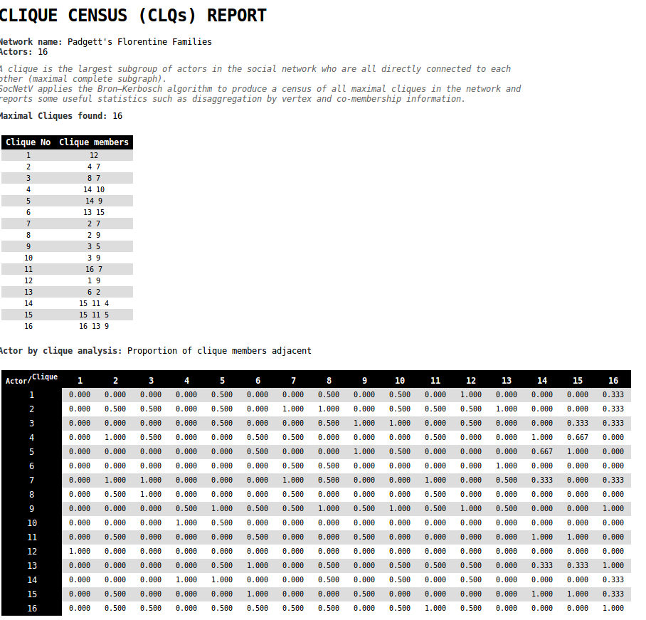
A clique is a group of people who interact with each other more regularly and intensely than with other people not belonging to the clique. In mathematical terms, a clique is a subset of vertices in an undirected graph $G$, where every two distinct vertices in the clique are adjacent to each other, forming a complete subgraph.

In Social Network Analysis, a clique refers to a maximal subgroup of actors who are all directly connected to each other. A maximal clique is a clique that cannot be extended by adding any further actor — all remaining actors are missing at least one tie to a current member. Maximal cliques may overlap (an actor can belong to more than one), and finding all of them reveals the dense sub-communities inside the network.

SocNetV computes a census of maximal cliques, producing:

• A list of all maximal cliques and their members.
• Per-actor clique membership counts.
• A co-membership matrix $CLQM$, where $CLQM_{ij}$ counts how many maximal cliques actors $i$ and $j$ share.

How it works — the Bron–Kerbosch algorithm with pivot selection

SocNetV implements the Bron–Kerbosch algorithm [1] with the Tomita et al. (2006) pivot selection heuristic [2].

The algorithm maintains three disjoint vertex sets at each recursive step:

Set	Meaning
R	The clique being built — all vertices in R are mutually adjacent
P	Candidates that can still extend R (each is adjacent to every vertex in R)
X	Vertices already processed that are also adjacent to every vertex in R — used to avoid reporting the same clique twice

When both P and X are empty, R is a maximal clique and is recorded.

Example: Consider a network with four actors — A, B, C, D — and edges A–B, A–C, B–C, and C–D:

graph LR A((A)) --- B((B)) A((A)) --- C((C)) B((B)) --- C((C)) C((C)) --- D((D)) style A fill:#4f86c6,color:#fff,stroke:#2d5f9e style B fill:#4f86c6,color:#fff,stroke:#2d5f9e style C fill:#e07b39,color:#fff,stroke:#b05a1e style D fill:#6aaa64,color:#fff,stroke:#4a8a44

The two maximal cliques are {A, B, C} (the triangle) and {C, D} (the edge, since D has no other neighbours).

Recursion trace:

Step	R	P	X	Action
Start	{}	{A,B,C,D}	{}	choose pivot C (most neighbours in P)
Branch C	{C}	{A,B,D}	{}	choose pivot A
Branch A	{C,A}	{B}	{}
Branch B	{C,A,B}	{}	{}	✅ clique {A,B,C}
Back to {C}	{C}	{A,B,D}	{A}	branch D
Branch D	{C,D}	{}	{}	✅ clique {C,D}

Why pivot selection matters

Without pivoting, the algorithm would iterate over every vertex in P at each level. For a network with many vertices and few cliques this produces an explosion of redundant recursive calls.

Tomita et al. (2006) proved that choosing a pivot vertex $u \in P \cup X$ that maximises $|N(u) \cap P|$ (the number of candidates that are neighbours of $u$) allows the main loop to only iterate over the non-neighbours of $u$ in P — the set $P \setminus N(u)$.

Why this is correct: any maximal clique that extends R must contain at least one vertex from $P \setminus N(u)$. If a clique contained only neighbours of $u$, it could be extended by $u$ itself (since $u$ is adjacent to all of them and to all of R), contradicting maximality.

Why this is faster: by choosing the pivot that maximises $|N(u) \cap P|$, we minimise $|P \setminus N(u)|$ — the number of branches at this level. In the example above, pivot C covers 3 out of 4 candidates, reducing the top-level loop from 4 iterations to just 1.

In practice this gives dramatic speedups on dense graphs and real-world social networks, where high-degree nodes cover most candidates.

Caution

Finding all maximal cliques is an NP-complete problem. Even with pivot selection, the computation can be slow on very large or highly connected networks, since the number of maximal cliques can itself be exponential. For networks with thousands of nodes and high density, expect long runtimes.

References

1. Bron, C. & Kerbosch, J. (1973). Algorithm 457: Finding all cliques of an undirected graph. Communications of the ACM, 16(9), 575–577.
2. Tomita, E., Tanaka, A. & Takahashi, H. (2006). The worst-case time complexity for generating all maximal cliques and computational experiments. Theoretical Computer Science, 363(1), 28–42. https://doi.org/10.1016/j.tcs.2006.06.015

---

Triad Census

A triad is a set of three nodes in a network. Triads are essential for understanding the local structure of a network, as they capture the relationships between three actors. In a network of $N$ actors, there are $C(N, 3) = 60$ possible triads, where $C(N, 3)$ represents the combination formula for selecting 3 nodes from $N$ actors:

$$C(N, 3) = \frac{N!}{3!(N-3)!}$$

The Triad Census is used to identify and count all possible types of triads in a network.

There are 16 different triad types (isomorphism classes), each labeled according to the M-A-N labeling scheme, as described by Holland, Leinhardt, and Davis, which categorizes the triads as follows:

• M: Number of mutual (M) dyads in the triad (possible values: 0, 1, 2, 3)
• A: Number of asymmetric (A) dyads in the triad (possible values: 0, 1, 2, 3)
• N: Number of null (N) dyads in the triad (possible values: 0, 1, 2, 3)
• Fourth character: Infers features such as cycle or transitivity (possible values: none, D (Down), U (Up), C (Cyclic), T (Transitive))

The following list shows all the 16 triad types:

Within each row, all the triad types have the same number of arcs present:

003
012
102     021D  021U  021C
111D    111U  030T  030C
201     120D  120U  120C
210
300

So, when you click on the Triad Census menu option, SocNetV calculates and displays a vector $T$ of length 16. Each element $T_u$ is the frequency of a specific triad type in the network, e.g., $T_{003} = 3$.

Furthermore, the order of the elements of vector T is the same as the aforementioned ordering of the triad types:

T = [ T003, T012, T102, T021D, T021U, T021C, T111D, T111U, T030T, T030C, T201, T120D, T120U, T120C, T210, T300 ]

The sum of all these frequencies equals $C(N,3)$, the total number of possible triads in the network.

---

Structural Equivalence Methods

A key notion in Social Network Analysis (SNA) is that of structural equivalence. The idea is to map the relationships in a graph by creating classes or groups of actors who are equivalent in some sense.

One way to identify these groups is by examining the relationships between actors for similarity patterns.

There are many methods to measure the similarity or dissimilarity of actors in a network.

SocNetV supports the following methods:

• Similarity by measure

• Pearson Correlation Coefficients

• Tie profile dissimilarities

By applying one of these methods, SocNetV creates a pairwise actor similarity/dissimilarity matrix.

Actor Similarity (by Measure)

This method computes a pairwise actor similarity matrix, where each element $(i, j)$ is the ratio of tie (or distance) matches of actors $i$ and $j$ to all other actors.

SocNetV supports the following measures:

• Simple Matching (Exact Matches): Proportion of tie/distance matches (present or absent) between two actors.

• Jaccard Index (Positive Matches or Co-citation): Percentage of same ties/distances reported by both actors to the total number of ties reported.

• Hamming Distance: Number of ties/distances that differ between each pair of actors.

• Cosine Similarity

• Euclidean Distance

For example, in the case of Simple Matching, the similarity matrix depicts the ratios of exact matches of pairs of actors to all other actors. If the element $(i, j) = 0.5$, it means that actors $i$ and $j$ have the same ties present or absent 50% of the time.

These measures of similarity are particularly useful when ties are binary (not valued).

Note

In very sparse networks (with low density), measures such as exact matches, correlation, and distance will show little variation among the actors, making it difficult to classify the actors into structural equivalence classes.

Pearson Correlation Coefficients

This method computes a correlation matrix, where the elements are the Pearson correlation coefficients between pairs of actors in terms of their tie profiles or distances (in, out, or both).

The Pearson product-moment correlation coefficient (PPMCC or PCC, or simply Pearson’s $r$) is a measure of the linear dependence or association between two variables $X$ and $Y$.

This correlation measure of similarity is particularly useful when ties are valued/weighted, denoting strength, cost, or probability.

Tie Profile Dissimilarities

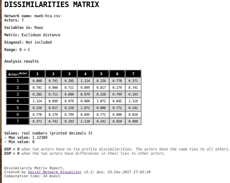
This method computes a matrix of tie profile distances/dissimilarities between all pairs of actors/nodes in the social network using an ordinary metric such as Euclidean distance, Manhattan distance, Jaccard distance, or Hamming distance.

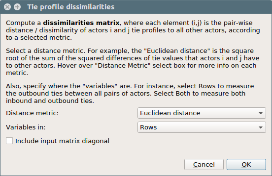
The resulting distance matrix is an $n \times n$ matrix, where the element $(i, j)$ is the distance or dissimilarity between the tie profiles of node $i$ and node $j$.

Hierarchical Cluster Analysis (HCA)

Hierarchical Clustering (or Hierarchical Cluster Analysis, HCA) is a method of cluster analysis that builds a hierarchy of clusters based on their elements’ dissimilarity. In the context of SNA, these clusters usually consist of network actors.

This method takes the social network distance matrix as input and uses the Agglomerative “bottom-up” approach, where each actor starts in its own cluster (Level 0). In each subsequent level, as we move up the clustering hierarchy, a pair of clusters are merged into a larger cluster, until all actors end up in the same cluster.

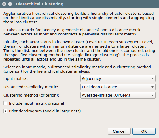
To decide which clusters should be combined at each level, a measure of dissimilarity between sets of observations is required. This measure consists of a metric for the distance between actors (e.g., Manhattan distance) and a linkage criterion (e.g., single-linkage clustering).

This linkage criterion (essentially a definition of distance between clusters) differentiates between the different HCA methods.

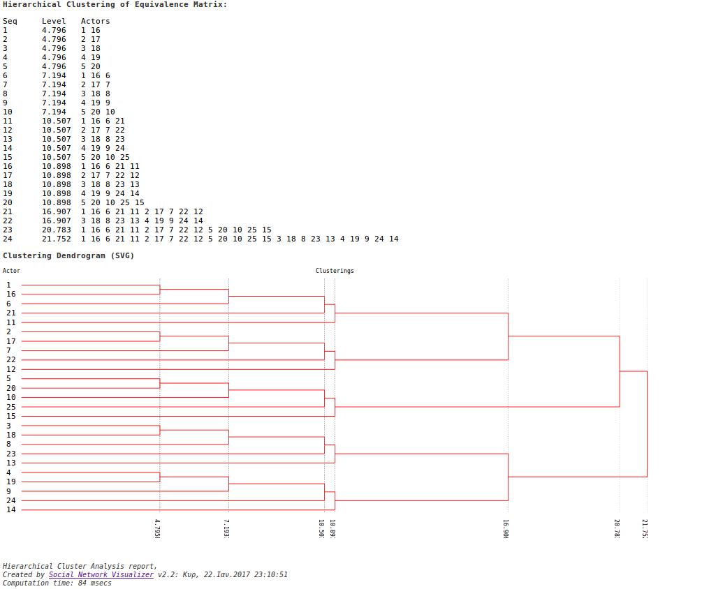
The result of Hierarchical Cluster Analysis is the clusters per level and a dendrogram:

Caution

The complexity of agglomerative clustering is $O(n^2 \log n)$, which makes it too slow for large data sets.