Supported Formats
SocNetV supports the following network data formats:
- GraphML (.graphml or .xml)
- GML (.gml or .xml)
- GraphViz (.dot)
- Adjacency Matrix (.sm, .adj, or .csv)
- Two-Mode Sociomatrix Files (.2sm)
- Pajek (.net, .paj, or .pajek)
- UCINET’s Data Language (.dl)
- Edge List (.lst or .list)
- Weighted Lists (.wlst or .wlist)
The default network data format of SocNetV is GraphML.
If you create a new network and press Ctrl+S to save it, SocNetV will try to save it in GraphML format by default.
In addition to the above graph topology formats, SocNetV v3.5 also supports structured CSV and JSON for exporting and importing node/edge attribute data via the Data Table dock. These are not graph formats — they carry attribute columns, not topology. See the Structured CSV and JSON section at the end of this page.
Loading and Importing Files
-
GraphML files can be loaded directly using
File > Loador specified via the command line. -
For other formats, use
File > Import.
GraphML files
GraphML is a highly versatile and widely adopted XML-based format designed for graph data representation. SocNetV supports both reading and saving networks in GraphML format, making it an excellent choice for interoperability with other network analysis tools.
| Import | ✅ File → Load or File → Import |
| Export | ✅ File → Save (default format) |
| Node labels | ✅ |
| Node colors / shapes | ✅ |
| Edge weights | ✅ |
| Edge labels | ✅ |
| Multiple relations | ✅ (via relation edge attribute) |
| Custom node / edge attributes | ✅ full roundtrip (d1000+ / d2000+ key ranges) |
Features of GraphML
- XML-Based: Uses XML structure to represent nodes, edges, and their attributes.
- Custom Attributes: Allows defining custom attributes for nodes and edges, such as labels, weights, or types. SocNetV v3.5 supports a full node and edge custom attribute roundtrip: arbitrary key/value pairs added in the Node Properties dialog or the Edge Properties dialog are saved and restored without loss. Node custom attribute keys use the
d1000+numbering range; edge custom attribute keys use thed2000+range (see Example 3 below). - Directed and Undirected Graphs: Supports both directed and undirected graph structures.
- Hierarchical Graphs: Facilitates multi-level graph representations.
- Multirelational Networks: SocNetV supports storing multiple relations between the same set of nodes by using edge attributes (for example a
relationattribute identifying the type of tie).
Examples
Example 1: A simple GraphML File
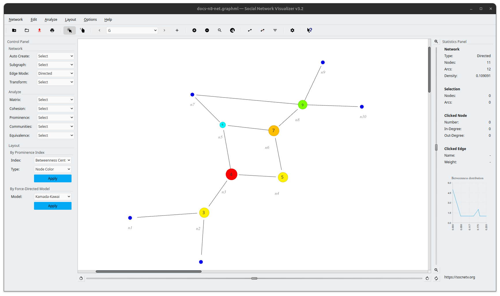
Below is an example of a simple social network in GraphML, an undirected graph with two 11 nodes and 12 edges:
<?xml version="1.0" encoding="UTF-8"?><graphml xmlns="http://graphml.graphdrawing.org/xmlns" xmlns:xsi="http://www.w3.org/2001/XMLSchema-instance" xsi:schemaLocation="http://graphml.graphdrawing.org/xmlns http://graphml.graphdrawing.org/xmlns/1.0/graphml.xsd"> <graph id="G" edgedefault="undirected"> <node id="n0"/> <node id="n1"/> <node id="n2"/> <node id="n3"/> <node id="n4"/> <node id="n5"/> <node id="n6"/> <node id="n7"/> <node id="n8"/> <node id="n9"/> <node id="n10"/> <edge source="n0" target="n2"/> <edge source="n1" target="n2"/> <edge source="n2" target="n3"/> <edge source="n3" target="n5"/> <edge source="n3" target="n4"/> <edge source="n4" target="n6"/> <edge source="n6" target="n5"/> <edge source="n5" target="n7"/> <edge source="n6" target="n8"/> <edge source="n8" target="n7"/> <edge source="n8" target="n9"/> <edge source="n8" target="n10"/> </graph></graphml>Explanation:
All GraphML files consist of a graphml element and a variety of sub-elements: graph, node, edge, keys. SocNetV understands all of them:
-
Nodes: Each
<node />element has an id attribute, which uniquely identifies the node. In this case, the nodes are labeled n0 through n10. -
Edges: Each
<edge />element defines a relationship between two nodes, indicated by source and target. For example,<edge source="n0" target="n2"/>indicates an edge from node n0 to node n2. -
Graph Structure: The graph is undirected as indicated by the
edgedefault="undirected"attribute in the<graph />element.
Here is the visualization of the above example using Mermaid, which demonstrates the directed graph structure:
And here’s the visualization of the above example using SocNetV where we have applied an FDP layout (Kamada-Kawai) for the node location and a prominence-based model (Betweenness Centrality) for the node sizes/colors:
Example 2: A multirelational GraphML network
GraphML can also represent multirelational networks, where multiple types of ties exist between the same actors.
In SocNetV, multirelational networks are stored by using multiple <graph> elements inside the same GraphML document, where each <graph> represents one relation (layer) of the network.
Example: a small network with two relations between the same actors.
<?xml version="1.0" encoding="UTF-8"?><graphml xmlns="http://graphml.graphdrawing.org/xmlns">
  <!-- Relation 1 -->  <graph id="relation_1" edgedefault="directed">    <node id="1"/>    <node id="2"/>    <node id="3"/>
    <edge source="1" target="2"/>    <edge source="2" target="3"/>  </graph>
  <!-- Relation 2 -->  <graph id="relation_2" edgedefault="directed">    <node id="1"/>    <node id="2"/>    <node id="3"/>
    <edge source="1" target="2"/>    <edge source="3" target="1"/>  </graph>
</graphml>
Explanation
- Each
<graph>element represents one relation in the multirelational network. - The same set of nodes may appear in multiple relations.
- The edges inside each
<graph>belong only to that specific relation. - When loaded in SocNetV, each
<graph>becomes a separate relation layer that can be selected, edited, or analyzed independently.
Visualization of the two relations:
Relation 1:
Relation 2:
Example 3: Node and Edge Custom Attributes
SocNetV v3.5 persists arbitrary custom attributes on both nodes and edges using GraphML <key> / <data> pairs. Node custom attribute keys are assigned IDs in the d1000+ range; edge custom attribute keys use the d2000+ range. This guarantees they never collide with SocNetV’s own built-in keys.
<?xml version="1.0" encoding="UTF-8"?><graphml xmlns="http://graphml.graphdrawing.org/xmlns"         xmlns:xsi="http://www.w3.org/2001/XMLSchema-instance"         xsi:schemaLocation="http://graphml.graphdrawing.org/xmlns         http://graphml.graphdrawing.org/xmlns/1.0/graphml.xsd">
  <!-- Built-in node attributes (SocNetV internal range) -->  <key id="d0" for="node" attr.name="label"  attr.type="string"/>  <key id="d1" for="node" attr.name="size"   attr.type="double"/>  <key id="d2" for="node" attr.name="color"  attr.type="string"/>
  <!-- Custom node attribute (d1000+ range) -->  <key id="d1000" for="node" attr.name="type"       attr.type="string"/>  <key id="d1001" for="node" attr.name="department"  attr.type="string"/>
  <!-- Built-in edge attributes (SocNetV internal range) -->  <key id="d100" for="edge" attr.name="weight" attr.type="double"/>  <key id="d101" for="edge" attr.name="label"  attr.type="string"/>
  <!-- Custom edge attributes (d2000+ range) -->  <key id="d2000" for="edge" attr.name="category" attr.type="string"/>  <key id="d2001" for="edge" attr.name="since"    attr.type="string"/>
  <graph id="G" edgedefault="directed">
    <node id="n1">      <data key="d0">Alice</data>      <data key="d1">10</data>      <data key="d2">#ff0000</data>      <data key="d1000">investor</data>      <data key="d1001">finance</data>    </node>
    <node id="n2">      <data key="d0">Bob</data>      <data key="d1">7</data>      <data key="d2">#0000ff</data>      <data key="d1000">manager</data>      <data key="d1001">operations</data>    </node>
    <edge source="n1" target="n2">      <data key="d100">2.5</data>      <data key="d101">funds</data>      <data key="d2000">partnership</data>      <data key="d2001">2022</data>    </edge>
  </graph></graphml>
Key points:
d1000/d1001are custom node attribute keys — added via the Node Properties dialog in SocNetV, or imported from CSV/JSON via the Data Table dock.d2000/d2001are custom edge attribute keys — added via the Edge Properties dialog.- On file load, SocNetV reads back all
d1000+andd2000+keys and populates the node/edge attribute tables without any data loss. - Keys in the built-in range (
d0–d999) are mapped to SocNetV’s internal properties (label, size, color, weight, etc.).
How to Use GraphML Files in SocNetV
Loading GraphML Files
To load a GraphML file in SocNetV:
- Go to File > Load.
- Select the desired
.graphmlfile. - The network will be rendered on the canvas with all its nodes, edges, and attributes.
Saving to GraphML files
To save a network as a GraphML file:
- Go to File > Save As.
- Choose the GraphML format from the list.
- Specify the filename and save.
Pros and Cons of GraphML
Advantages:
- Standardized Format: As an XML-based format, GraphML is standardized and widely supported by many graph-analysis tools (such as SocNetV, Cytoscape, yEd, etc) making it easy to exchange graph data.
- Extensible and Flexible: With support for custom attributes, GraphML is highly flexible and can describe complex networks with rich metadata.
- Schema Validation: GraphML supports schema validation, allowing users to ensure that graph data adheres to a predefined structure, which is useful for maintaining data integrity.
- Supports Multirelational Networks: By using edge attributes, GraphML can represent multiple types of relations between actors.
Disadvantages:
- File Size: Since GraphML is an XML-based format, it can be larger in size compared to binary formats, especially for large graphs. This can make file handling and transfer slower.
- Complexity for Simple Graphs: For simpler, smaller networks, GraphML may be overkill compared to simpler formats like GML or CSV, which may be easier to use for basic graph tasks.
- Parsing Overhead: Parsing XML can be more computationally expensive than parsing other formats, especially when working with large graphs, potentially affecting performance.
Reference
- GraphML Official Specification: GraphML Specification
GML Files
GML (Graph Modeling Language) is a simple, text-based file format designed for describing graphs. It is widely used due to its human-readable structure and its ability to represent both small and large graphs in a flexible way. GML files are commonly used for storing and exchanging graph data and are supported by many graph-processing tools, including SocNetV.
| Import | ✅ File → Import |
| Export | ❌ not supported |
| Node labels | ✅ (via label attribute) |
| Node colors / shapes | ❌ not parsed |
| Edge weights | ✅ (via value attribute) |
| Multiple relations | ❌ |
| Custom node / edge attributes | ❌ |
Features of GML
- Human-readable format: GML is a text-based format that is easy to read and edit manually, making it accessible even to users without specialized graph software.
- Flexibility in Graph Representation: GML supports both directed and undirected graphs, as well as the inclusion of additional attributes for nodes and edges, such as labels, weights, and other custom properties.
- Graph-Level Properties: GML allows you to define global properties for the graph, such as directionality, making it easy to specify the overall structure of the network.
Examples
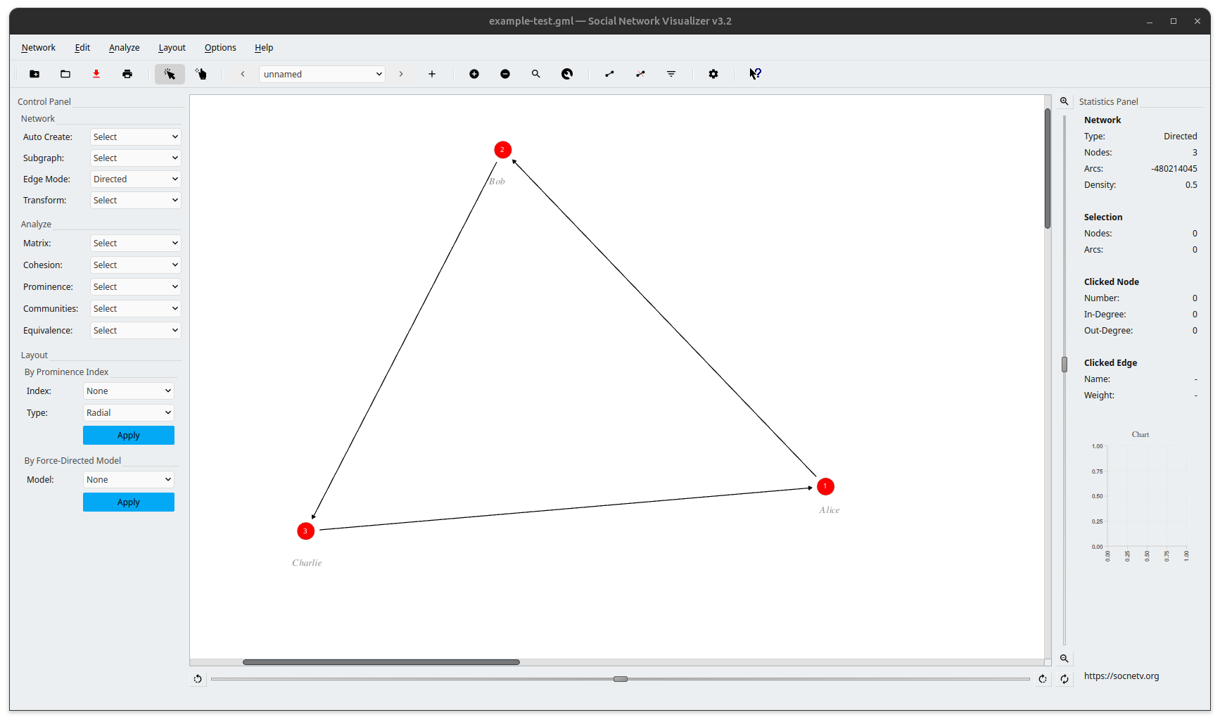
Example 1: A simple GML File
graph [ directed 1 node [ id 1 label "Alice" ] node [ id 2 label "Bob" ] node [ id 3 label "Charlie" ] edge [ source 1 target 2 weight 1.0 ] edge [ source 2 target 3 weight 0.5 ] edge [ source 3 target 1 weight 2.0 ]]Explanation
- Nodes: Each node is defined by an
id(unique identifier) and an optionallabelthat describes the node. In this example, three nodes are defined: “Alice”, “Bob”, and “Charlie”, each with a unique ID. - Edges: The edges connect nodes using the
sourceandtargetattributes. For example, an edge from node1(Alice) to node2(Bob) has a weight of1.0. Similarly, other edges are defined with weights that indicate the strength of the connection. - Graph Properties: The
directed 1property at the beginning of the graph indicates that the graph is directed. If this value were set to0, the graph would be undirected.
Visualization
This Mermaid diagram visualizes the directed graph described in the GML example. It captures the relationships between “Alice”, “Bob”, and “Charlie”, along with the weights assigned to the edges.
And here’s the visualization in SocNetV:
How to Use GML in SocNetV
- Loading GML Files: In SocNetV, you can load a GML file by selecting File > Import from the menu and choosing your GML file. SocNetV will parse the file and display the network graph, preserving node labels, edge weights, and any other attributes defined in the GML.
- Saving Networks as GML: Exporting a network from SocNetV in the GML format is not supported.
Supported GML Elements in SocNetV
SocNetV supports the following key features of GML files:
- Graph Type: Directed (
directed 1) and undirected graphs (directed 0). - Node Attributes:
id,label, and simple custom attributes such ascolororsizefor nodes. - Edge Attributes:
source,target, and simple attributes likeweightandcolorfor edges. - Basic Graph Structure: SocNetV can handle simple graph structures with nodes and edges but does not support hierarchical elements or advanced GML features like nested graphs.
Pros and Cons of GML
Advantages:
- Human-readable: As a text-based format, GML files are easy to read and edit by hand, making it simple to inspect and modify graph data.
- Wide tool support: Many graph analysis tools, including SocNetV, support GML, making it a versatile format for sharing and processing graphs.
- Flexibility: GML allows the inclusion of various attributes for both nodes and edges, making it adaptable to different types of networks.
Disadvantages:
- Scalability Issues: For very large graphs, GML can become inefficient because it is a text-based format, leading to larger file sizes and slower parsing times compared to binary formats.
- Limited Structure: While GML is flexible, it lacks the extensive validation or schema enforcement seen in more structured formats, which can lead to inconsistencies in large, complex graphs.
- Manual Edits Can Be Error-Prone: While human-readable, manual edits to a GML file can easily introduce syntax errors or formatting mistakes, especially in large graphs.
Reference
- GML Official Specification: Graph Modeling Language (GML) Specification
GraphViz (DOT) Files
GraphViz is a graph description language that uses the “DOT format” to define and represent graphs. SocNetV supports importing GraphViz files for analysis and visualization. These files describe graphs using a simple text-based syntax, making them easy to create and edit.
| Import | ✅ File → Import |
| Export | ✅ Network → Export → GraphViz DOT |
| Graph types | graph (undirected) · digraph (directed) · strict variants |
| Node labels | ✅ |
| Node colors / shapes | ✅ (color, shape, pos attributes) |
| Edge weights | ✅ (weight attribute) |
| Edge labels | ✅ (label attribute) |
| Multiple relations | ❌ active relation only |
| Custom node / edge attributes | ✅ arbitrary key=value pairs roundtrip via pos= and unknown attrs |
| Subgraph / cluster hierarchy | ❌ structure parsed but not preserved as entities |
Key Features
- Directed and Undirected Graphs: GraphViz supports both graph types using intuitive syntax (
digraphfor directed graphs andgraphfor undirected graphs). SocNetV determines the graph type directly from this declaration. - Attribute Definitions: Customize nodes and edges with attributes like colors, shapes, labels, and weights to enrich graph visualizations.
- Hierarchical Structures: GraphViz allows defining subgraphs and clusters. SocNetV parses the graph structure but does not preserve cluster or subgraph hierarchy as structural entities.
Examples
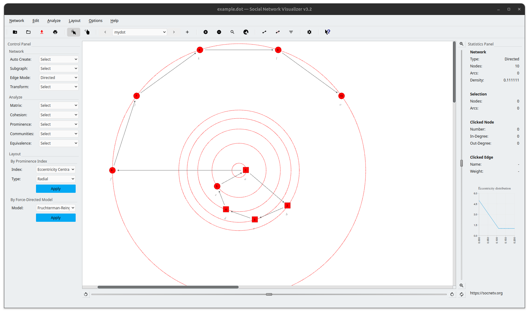
Example 1 : A simple .dot file
digraph mydot { node [color=red, shape=box]; a -> b -> c -> d; node [color=pink, shape=circle]; d -> e -> a -> f -> j -> k -> l -> o [weight=1, color=black];}Explanation
- Graph Type: The keyword
digraphindicates a directed graph, where edges have direction. If the file begins withgraph, SocNetV treats it as undirected. - Node Attributes: Nodes can have attributes such as
colorandshape. SocNetV applies supported visual attributes during import. - Edges: Directed edges are defined using
->, while undirected edges use--. Attributes likeweight,color, andlabelcan also be applied to edges. - Attribute Blocks: Default node or edge attributes declared at block level are applied to subsequent elements where supported.
Visualization:
This Mermaid diagram replicates the structure of the example GraphViz file, illustrating the directed relationships between nodes.
In SocNetV, the same network can be visualized in many ways. For instance, in the screenshot below, we have applied a prominence-based layout (Eccentricity):
How to Use GraphViz Files in SocNetV
Importing GraphViz DOT Files
- Navigate to File > Import and select the
.dotfile. - SocNetV renders supported attributes (node colors, shapes, labels, edge weights). Unsupported or unrecognized attributes are safely ignored.
- Limitations: SocNetV does not support advanced GraphViz features such as full cluster layout control, subgraph hierarchy preservation, or complex attribute inheritance rules.
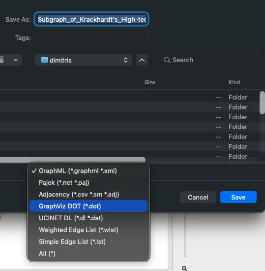
Exporting to GraphViz DOT
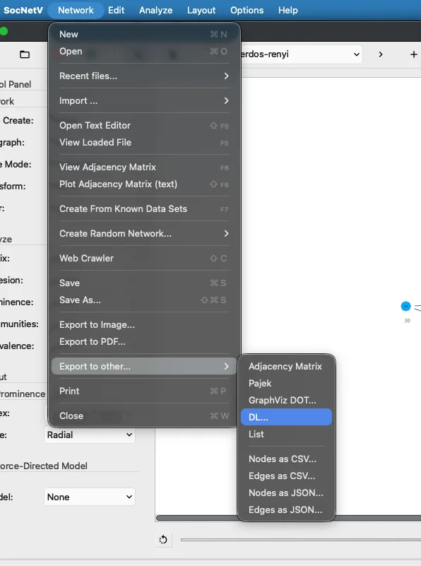
Go to Network → Export to other… → GraphViz DOT… to save the current graph in DOT format.
What is exported:
- Node labels, colors, and shapes as DOT node attributes.
- Edge weights, labels, and colors as DOT edge attributes.
- Custom node and edge attributes as additional DOT key/value pairs.
- Node canvas positions as
pos="x,y"attributes, enabling a lossless positional roundtrip — reload the exported.dotfile to restore the same layout.
Limitations:
- Only the active relation is exported (single
digraphorgraphblock). Multi-relation networks require one export per relation. - Advanced DOT layout directives (e.g.,
rankdir,splines) are not written.
Supported DOT Elements in SocNetV
SocNetV supports the following core elements of GraphViz files:
- Graph Type:
digraph(directed) andgraph(undirected). - Edge Syntax:
->for directed edges and--for undirected edges. - Node Attributes:
color,shape,label, and basic styles such asfillcolorandstyle. - Edge Attributes:
weight,color, andlabel. - Basic Structure: Node and edge declarations are parsed and converted into SocNetV’s internal graph model.
Subgraphs and clusters may be parsed for structural correctness, but their hierarchical semantics are not preserved.
Pros and Cons of GraphViz Files
Advantages:
- Human-Readable Syntax: Easy to create and edit with any text editor.
- Customizable: Allows detailed customization of nodes and edges using attributes.
- Widely Supported: Used in many visualization tools, including SocNetV.
Disadvantages:
- Partial Feature Support: SocNetV does not implement the full DOT specification, especially advanced layout or cluster semantics.
- Formatting Sensitivity: Requires properly formatted DOT syntax; malformed files may fail to import.
- Visualization Complexity: Large graphs with extensive attributes can become difficult to manage and interpret.
Reference:
- GraphViz Official Documentation: GraphViz DOT Language
Adjacency Matrix Files
The adjacency matrix format is a widely used format for representing one-mode networks, where each element in an NxN matrix represents the connection between nodes (or the weight). This format is simple to use and is typically employed for analyzing networks based on node relationships.
SocNetV supports adjacency matrix files with extensions .sm, .adj, and .csv.
| Import | ✅ File → Import |
| Export | ✅ Network → Export → Adjacency Matrix |
| Matrix shape | Square N × N (one-mode only) |
| Node labels | ✅ optional — first #-comment line, comma-separated |
| Edge weights | ✅ any non-zero numeric cell value |
| Multiple relations | ❌ active relation only |
| Node colors / shapes | ❌ not in format |
| Custom node / edge attributes | ❌ not in format |
Key Features
- Each line in the matrix corresponds to a row, and the entries are separated by a delimiter: a space, a comma, a tab etc.
- The value at position
(i, j)in the matrix represents the weight of the edge from nodeito nodej. For unweighted networks, use1for edges and0for no connection. - Diagonal elements (self-loops) can be included but are not mandatory.
- Directed networks can be represented by an asymmetric adjacency matrix, where the entry
(i, j)differs from(j, i).
Node Labels
In addition to numeric node identifiers, SocNetV supports labeled nodes. This feature enables users to define custom node labels, making the matrix more descriptive.
Labels can be provided as follows:
- A header comment line at the top of the file lists the node labels, separated by spaces or tabs.
- The subsequent rows represent the adjacency matrix, where the order of rows matches the order of node labels.
Examples
Example 1: Adjacency Matrix File with Numeric Node Identifiers
For a simple network:
0 1 01 0 10 1 0Explanation:
- Matrix Representation: Each row and column in the matrix represents a node. The element
(i, j)represents the connection between nodeiand nodej. For example, the first row (0 1 0) means node 1 is connected to node 2 - Unweighted: In this example, the matrix is unweighted, with binary values (0 and 1).
- Symmetry: The adjacency matrix is symmetric for undirected graphs, meaning
A[i][j] = A[j][i].
Example 2: With Labeled Nodes
Using labels instead of numeric identifiers:
# Alice Bob Carol0 1 01 0 11 0 0Here:
Aliceis connected toBob.Bobis connected to bothAliceandCarol.Carolis connected toAlice.
Note that this matrix is not symmetric.
This format is especially useful for social networks where nodes represent entities like people, organizations, or websites, and meaningful labels enhance readability.
Example 3: A Weighted Network
0, 1, 1, 21, 0, 2, 10, 0, 0, 11, 0, 0, 0Explanation:
- Matrix Representation: Each row and column in the matrix represents a node. The element
(i, j)represents the connection between nodeiand nodej. For example, the first row (0, 1, 1, 2) means node 1 is connected to node 2 (with weight 1), and node 3 (with weight 1), while node 4 is connected to node 1 (with weight 2). - Weighted: In this example, the matrix is weighted, with values like 1 and 2 indicating the strength of the connections. Unweighted matrices would use binary values (0 and 1).
- Symmetry: The adjacency matrix is symmetric for undirected graphs, meaning
A[i][j] = A[j][i].
Visualization:
This Mermaid diagram visualizes the graph represented by the adjacency matrix. The nodes 1, 2, 3, and 4 are connected with weighted edges, as indicated by the matrix.
How to Use Adjacency Matrix Files in SocNetV
- Loading Files: In SocNetV, you can load an adjacency matrix file by selecting the File > Import > Adjacency Matrix menu option. and choosing the appropriate file. SocNetV will parse the matrix and display the graph, representing each node and its connections.
- Delimiters: When importing an adjacency matrix, SocNetV allows you to specify the delimiter used in the file (comma, space, or tab) for correct parsing.
- Exporting as Matrix: SocNetV allows exporting the graph as an adjacency matrix file, which can be shared and used in other tools for further analysis.
Supported Elements in SocNetV
SocNetV supports the following elements of adjacency matrix files:
- Basic Structure: The matrix should be a square matrix (NxN), where
Nis the number of nodes in the network. - Weighted and Unweighted Networks: SocNetV can handle both weighted (non-zero values) and unweighted (binary values 0 and 1) networks.
- Node Labels: SocNetV supports the inclusion of node labels, either in the comment line (e.g.,
# Alice, Bob, Charlie) or as part of the matrix input.
Pros and Cons of Adjacency Matrix Files
The Adjacency Matrix Format is widely used in research and applications where the network structure is predefined, such as importing datasets from external tools or simulations. The inclusion of labels further enhances its versatility for descriptive and real-world social network data.
Advantages:
- Simple and Efficient: Adjacency matrices are straightforward to use and understand, especially for small networks or those without complex structures.
- Widely Supported: The matrix format is widely accepted and can be used across various graph analysis and network tools.
- Direct Representation of Connections: The matrix provides an explicit representation of node connections, which is useful for mathematical and algorithmic analysis of networks.
Disadvantages:
- Scalability Issues: For large networks, the adjacency matrix can become inefficient in terms of both storage and processing. Sparse networks can lead to a lot of wasted space in memory.
- Limited Metadata: The adjacency matrix format is not ideal for representing additional information (e.g., node attributes) beyond connections. While it supports weights, more complex node and edge attributes are difficult to handle in this format.
- Not Ideal for Directed Graphs: While the matrix can represent directed graphs, it becomes more difficult to distinguish between directed and undirected edges without additional context.
Reference:
- Adjacency Matrix Files: Adjacency Matrix Explanation (Wikipedia)
Two-Mode Sociomatrix Files
A two-mode sociomatrix represents bipartite networks — networks where two fundamentally different types of actors exist, and connections only occur between types, never within them. Classic examples include people and the organisations they belong to, authors and the papers they co-authored, or directors and the company boards they sit on.
SocNetV supports two-mode sociomatrix files with extensions .2sm and .aff.
| Import | ✅ File → Import — dialog lets you choose import mode |
| Export | ❌ not supported |
| Matrix shape | Rectangular NR × NC (Mode-1 rows × Mode-2 columns) |
| Import modes | Bipartite graph (NR+NC nodes) · Person network (NR nodes, B×Bᵀ projection) · Event network (NC nodes, Bᵀ×B projection) |
| Node labels | ❌ auto-labelled p1…pNR and e1…eNC in bipartite mode |
| Edge weights | ✅ any non-zero cell value treated as affiliation weight |
| Multiple relations | ❌ |
| Node colors / shapes | Mode-2 nodes styled as blue diamonds in bipartite mode |
| Comments | ✅ lines beginning with # are ignored |
Understanding Two-Mode Data
In a regular (one-mode) network, you have one type of actor. The adjacency matrix is square: rows and columns are the same set of nodes, and cell A[i][j] = 1 means node i is directly connected to node j.
A two-mode network has two distinct sets of actors — traditionally called Mode 1 (e.g. persons, CEOs, authors) and Mode 2 (e.g. events, clubs, papers). The raw data is a rectangular NR × NC matrix — NR rows for Mode 1 actors, NC columns for Mode 2 actors. A cell value of 1 (or any non-zero weight) means person i is affiliated with event j. Crucially, there are no direct person-to-person or event-to-event connections in the raw data — only person-to-event affiliations.
This rectangular matrix is richer than it looks. From it, three distinct graphs can be derived:
| Import mode | What you get | Nodes | Edges |
|---|---|---|---|
| Bipartite graph (default) | The raw affiliation graph | NR + NC | One per non-zero cell |
| Person network | Who shares a group with whom | NR | Person i — person k if they share ≥1 event |
| Event network | Which groups share members | NC | Event j — event l if they share ≥1 person |
SocNetV will ask you which of these three graphs to construct when you load a .2sm file.
Key Features
- The matrix is rectangular (NR × NC), not square. Rows = Mode 1 actors, columns = Mode 2 actors.
- Cell values can be binary (
0/1) or weighted (any non-zero numeric value representing affiliation strength). - Rows are separated by newlines. Values within a row are separated by spaces or commas.
- Comment lines beginning with
#are ignored. - In bipartite mode, Mode 1 nodes are labelled
p1…pNRand Mode 2 nodes are labellede1…eNC. Mode 2 nodes are visually distinct (blue diamond shape) so the two sets are immediately recognisable on the canvas.
Examples
Example 1: A Simple Bipartite Network
Four persons (rows) and three events (columns):
1 1 01 0 10 1 10 1 0Explanation:
- Person 1 attended events 1 and 2.
- Person 2 attended events 1 and 3.
- Person 3 attended events 2 and 3.
- Person 4 attended event 2 only.
Bipartite graph (default import): SocNetV creates 4 + 3 = 7 nodes and 7 edges (one per 1 in the matrix). Nodes p1–p4 represent persons; nodes e1–e3 represent events.
Person network (import mode 2): SocNetV creates 4 nodes and connects persons who share at least one event:
- p1–p2 share event 1
- p1–p3 share event 2
- p1–p4 share event 2
- p2–p3 share event 3
- p3–p4 share event 2
Event network (import mode 3): SocNetV creates 3 nodes and connects events that share at least one person:
- e1–e2 share person 1
- e1–e3 share person 2
- e2–e3 share person 3
Example 2: A Weighted Two-Mode Sociomatrix
Affiliation strength can be expressed with non-zero weights:
3 0 10 2 21 1 0Explanation:
- Person 1 has a strong affiliation (weight 3) with event 1, and a weak affiliation (weight 1) with event 3.
- Person 2 has affiliation weight 2 with both events 2 and 3.
- Person 3 has affiliation weight 1 with events 1 and 2.
In bipartite mode, edge weights from the matrix are preserved. In person and event projection modes, edges are unweighted (presence/absence of co-membership only).
Example 3: The Galaskiewicz CEOs and Clubs Dataset
The shipped dataset Galaskiewicz_CEOs_and_clubs_affiliation_network_data.2sm is a real-world example — 26 CEOs (rows) × 15 clubs (columns):
0 0 1 1 0 0 0 0 1 0 0 0 0 0 00 0 1 0 1 0 1 0 0 0 0 0 0 0 00 0 1 0 0 0 0 0 0 0 0 1 0 0 00 1 1 0 0 0 0 0 0 0 0 0 0 0 10 0 1 0 0 0 0 0 0 0 0 0 1 1 00 1 1 0 0 0 0 0 0 0 0 0 0 1 00 0 1 1 0 0 0 0 0 1 1 0 0 0 00 0 0 1 0 0 1 0 0 1 0 0 0 0 01 0 0 1 0 0 0 1 0 1 0 0 0 0 00 0 1 0 0 0 0 0 1 0 0 0 0 0 00 1 1 0 0 0 0 0 1 0 0 0 0 0 00 0 0 1 0 0 1 0 0 0 0 0 0 0 00 0 1 1 1 0 0 0 1 0 0 0 0 0 00 1 1 1 0 0 0 0 0 0 1 1 1 0 10 1 1 0 0 1 0 0 0 0 0 0 1 0 10 1 1 0 0 1 0 1 0 0 0 0 0 1 00 1 1 0 1 0 0 0 0 0 1 1 0 0 10 0 0 1 0 0 0 0 1 0 0 1 1 0 11 0 1 1 0 0 1 0 1 0 0 0 0 0 00 1 1 1 0 0 0 0 0 0 1 0 0 0 10 0 1 1 0 0 0 1 0 0 0 0 0 0 00 0 1 0 0 0 0 1 0 0 0 0 0 0 10 1 1 0 0 1 0 0 0 0 0 0 0 0 11 0 1 1 0 1 0 0 0 0 0 0 0 0 10 1 1 0 0 0 0 0 0 0 0 0 1 0 00 1 1 0 0 0 0 0 0 0 0 1 0 0 0Importing as a bipartite graph produces 41 nodes (26 CEOs + 15 clubs) and one edge per club membership. Importing as a person network reveals which CEOs move in the same social circles. Importing as an event network reveals which clubs attract overlapping memberships.
How to Use Two-Mode Sociomatrix Files in SocNetV
-
Loading files: Select File > Import > Two-Mode Sociomatrix and choose your
.2smor.afffile. SocNetV will display a dialog asking which graph to construct. -
Choosing the import mode:
- Bipartite graph — recommended as the starting point. Preserves all information from the file. Both sets of actors appear as nodes; Mode 2 nodes are shown in blue diamond shape.
- Person network — use when you want to analyse relationships among the Mode 1 actors (e.g. which CEOs are socially proximate).
- Event network — use when you want to analyse relationships among the Mode 2 actors (e.g. which clubs attract overlapping memberships).
-
Delimiter: values within each row may be separated by spaces or commas — SocNetV detects both automatically.
Supported Elements in SocNetV
| Element | Supported |
|---|---|
| Rectangular NR × NC matrix | ✅ |
| Binary (0/1) affiliations | ✅ |
| Weighted affiliations | ✅ (bipartite mode) |
| Space-delimited rows | ✅ |
| Comma-delimited rows | ✅ |
Comment lines (#) | ✅ |
| Bipartite graph import | ✅ |
| Person projection import | ✅ |
| Event projection import | ✅ |
| Node labels in file | ❌ (not yet supported) |
Export back to .2sm | ❌ (not yet supported) |
Pros and Cons of Two-Mode Sociomatrix Files
Advantages
- Information-rich: a single file encodes three different graphs simultaneously, depending on how you choose to import it.
- Compact: for sparse affiliation data, a rectangular binary matrix is much smaller than an equivalent adjacency matrix covering all actors.
- Standard format: widely used in social network analysis research, with many published datasets available in this format (Davis Southern Women, Galaskiewicz CEOs and Clubs, etc.).
Disadvantages
- No node attributes: the format carries no metadata beyond the affiliation values themselves.
- Projection information loss: the person and event projection modes discard affiliation weights and merge co-memberships into a simple binary edge — some analytical nuance is lost.
- Export not yet supported: SocNetV can import
.2smfiles but cannot currently export a network back to this format.
References
- Wasserman, S. & Faust, K. (1994). Social Network Analysis: Methods and Applications. Cambridge University Press. — the standard reference for two-mode network analysis.
- Bipartite graph — Wikipedia
- Davis, A., Gardner, B. B., & Gardner, M. R. (1941). Deep South. University of Chicago Press. — source of the classic Southern Women two-mode dataset.
- Galaskiewicz, J. (1985). Social Organization of an Urban Grants Economy. Academic Press. — source of the CEOs and Clubs dataset shipped with SocNetV.
Pajek Files
SocNetV supports importing Pajek project files, which usually have a .net or .paj extension. It is important to note that SocNetV supports a limited subset of the features of this format.
| Import | ✅ File → Import |
| Export | ✅ Network → Export → Pajek |
| Sections | *Vertices · *Arcs · *Edges · *ArcsList · *Matrix |
| Node labels | ✅ |
| Node colors / shapes | ✅ (ic, shape keywords, canvas coordinates) |
| Edge weights | ✅ |
| Multiple relations | ✅ multiple *Matrix blocks, each imported as a separate relation |
| Custom node / edge attributes | ❌ |
| Pajek features not supported | Partitions, vectors, permutations, cluster files |
Key Features
-
Network Definition: Pajek files start with the
*Networktag to declare the network and provide its name. -
Vertices and Edges/Arcs: The
*Verticessection lists nodes, and the*Edgesor*Arcssection defines relationships between nodes. -
ArcsList: The
*ArcsListtag is used to represent arcs from one node to others in a more compact form. SocNetV supports this tag for defining relationships in a simplified way. -
Matrix Representation: SocNetV can also handle Pajek files that use the
*Matrixtag to represent relationships in an adjacency matrix format. -
Multiple Matrix Declarations: SocNetV supports files with multiple
*Matrixtags, which will each be parsed as a separate relation within the same network. -
Canonical Matrix Export: When exporting multirelational networks, SocNetV writes matrix headers in canonical Pajek form:
*Matrix :k*Matrix :k "Label"
Examples
Example 1: A Simple Pajek Network
*Network "Simple Network"*Vertices 61 "pe0" ic LightGreen 0.5 0.5 box2 "pe1" ic LightYellow 0.8473 0.4981 ellipse3 "pe2" ic LightYellow 0.6112 0.8387 triangle4 "pe3" ic LightYellow 0.201 0.7205 diamond5 "pe4" ic LightYellow 0.2216 0.2977 ellipse6 "pe5" ic LightYellow 0.612 0.1552 circle*Arcs1 2 1 c black1 3 -1 c red2 4 1 c black3 5 1 c black*Edges6 4 1 c black5 6 1 c yellowExplanation:
- Network Declaration: The
*Networktag declares the name of the network, in this case, “Simple Network.” - Vertices: The
*Verticessection defines 6 nodes, each with an ID, a label (node name), color (LightGreen,LightYellow), and additional properties such as shape (box,ellipse, etc.) and position coordinates (0.5 0.5for the X and Y coordinates). - Arcs: The
*Arcssection defines directed edges between nodes. Each line specifies a source node, target node, weight (e.g.,1,-1), and an optional color. - Edges: The
*Edgessection defines undirected edges, similar to*Arcs, with the same format.
Visualization:
This Mermaid diagram visualizes the graph described in the Pajek file, showing the directed and undirected relationships between nodes.
Handling Multiple Matrices in Pajek Files
SocNetV supports Pajek files with multiple *Matrix declarations. Each matrix defines a new relation between the nodes.
Below is an example of a Pajek file with multiple matrices:
*Network "4 possible graphs of N=5"*Vertices 51 "1" ic red 0.221583 0.644042 circle2 "2" ic red 0.233094 0.351433 circle3 "3" ic red 0.696403 0.328808 circle4 "4" ic red 0.471942 0.197587 circle5 "5" ic red 0.726619 0.644042 circle*Matrix :10 0 0 0 00 0 0 0 00 0 0 0 00 0 0 0 00 0 0 0 0*Matrix :20 0 0 0 00 0 0 1 00 0 0 0 00 1 0 0 00 0 0 0 0*Matrix :30 1 0 0 01 0 0 1 00 0 0 0 00 1 0 0 00 0 0 0 0*Matrix :40 0 0 0 10 0 0 1 00 0 0 0 00 1 0 0 01 0 0 0 0Explanation:
- Multiple Matrices: Each
*Matrixsection represents an adjacency matrix that defines a relation between nodes. - Matrix Format: Each matrix is a square matrix (NxN), where
Nis the number of nodes in the network. The values inside the matrix represent the connections between the nodes, where0indicates no connection and any non-zero number (such as1or-1) represents a connection. - Multiple Relations: Each matrix is treated as a separate relation within the same network.
Matrix Header Compatibility
SocNetV is tolerant when importing matrix headers and accepts common real-world variants, including:
*Matrix :1*Matrix :1 "Label"*Matrix 1:*Matrix 1: "Label"During import:
- The matrix index (
1,2, etc.) is used only to determine the relation order. - If a label is present, it becomes the relation name.
- The index is not treated as part of the relation name.
- If no label is provided, SocNetV temporarily uses the matrix index as a relation name in the user interface.
During export:
-
SocNetV always writes matrix headers in canonical form:
*Matrix :k*Matrix :k "Label"
-
If a relation has no explicit label (only a temporary numeric name), it is exported as:
*Matrix :k(without writing
"k"as a quoted label).
This ensures deterministic round-trip behavior for multirelational Pajek files.
How to Use Pajek Files in SocNetV
- Loading Files: To import a Pajek file, navigate to File > Import and select the
.netor.pajfile. SocNetV will parse the file and display the network structure. - Limitations: SocNetV does not support advanced Pajek features like vectors, permutations, or event-based files.
Supported Pajek Elements in SocNetV
SocNetV supports the following elements of Pajek files:
- Network Declaration:
*Networkheader to define the start of the network file. - Node Definitions:
*Verticesfollowed by a list of nodes with their labels, colors, shapes, and optional positions. Node labels must be enclosed in double quotes (e.g. 1 “Alice Smith”); unquoted multi-word labels are ambiguous and will be parsed incorrectly. - Edge Definitions:
*Arcsfollowed by pairs of node IDs indicating directed connections, with optional weights and colors. - Edge Definitions:
*Edgesfor undirected relationships between nodes. - ArcsList: The
*ArcsListtag for representing multiple outgoing edges from a node in compact form. - Matrix Representation: The
*Matrixtag for adjacency matrices, including multiple matrices corresponding to multiple relations.
Pros and Cons of Pajek Files (in SocNetV)
Advantages:
- Simple Structure: Pajek files have a straightforward text-based format.
- Efficient for Large Networks: Designed for handling large graphs efficiently.
- Widely Used: Compatible with many network analysis tools.
Disadvantages:
- Limited Attribute Support: While Pajek files support some attributes, SocNetV handles a limited subset of visual and advanced attributes.
- Partial Feature Support: More complex Pajek constructs (e.g., vectors, permutations, event-based files) are not supported.
- No Schema Validation: Pajek files are not automatically schema-validated, so malformed files may cause import issues.
References
- Pajek File Format Documentation: Pajek Documentation
UCINET DL Files
UCINET’s DL (Data Language) format is widely used for representing social networks and other types of relational data. It is a simple and flexible text-based format, primarily designed for use with the UCINET software. SocNetV supports importing DL files as full matrices (FULLMATRIX), edge lists (EDGELIST1), and two-mode affiliation matrices (NR × NC).
| Import | ✅ File → Import |
| Export | ✅ Network → Export → UCINET DL |
| Format variants | FULLMATRIX · EDGELIST1 · Two-mode (NR × NC) |
| Node labels | ✅ LABELS / ROW LABELS / COLUMN LABELS / COL LABELS |
| Edge weights | ✅ matrix cell values or edge-list weight column |
| Multiple relations | ✅ NM=k header with sequential matrix blocks and optional LEVEL LABELS |
| Two-mode networks | ✅ always loads as a bipartite directed graph (see Example 1c) |
| Node colors / shapes | ❌ not in DL format |
| Custom node / edge attributes | ❌ not in DL format |
Key Features
- File Header: DL files start with the
DLkeyword, followed by metadata describing the number of nodes (N=), whether diagonals are present, and the data format. - Matrix or Edge List Representation: SocNetV supports
FULLMATRIX(adjacency matrix) andEDGELIST1(source–target–weight triples) formats. - Two-Mode Networks: Files that declare
NR=andNC=instead ofN=are treated as affiliation (bipartite) networks. - Node Labels: DL files can include node labels via
LABELS,ROW LABELS,COLUMN LABELS, orCOL LABELSsections.
Examples
Example 1a: Full Matrix Format
DLN=4FORMAT=FULLMATRIX DIAGONAL PRESENTLABELS:AliceBobCharlieDavidDATA:0 1 1 21 0 2 10 0 0 11 0 0 0Explanation:
- Header: The file starts with
DL, indicating the UCINET format, and specifies the number of nodes (N=4), the format (FULLMATRIX), and whether the diagonal is present. - Labels: The
LABELSsection lists the names of the nodes (e.g., Alice, Bob, Charlie, David). - Data: The
DATAsection provides the adjacency matrix for the network. For instance, the value1at position(1, 2)indicates a connection between Alice and Bob, with a weight of1.
Visualization:
This diagram visualizes the relationships described in the full matrix format, showing both the weights and the direction of edges.
Example 1b: Multirelational Full Matrix (Multiple Matrices)
UCINET DL files can also represent multirelational networks by including multiple matrices in the same file.
In this case, the header uses the parameter NM (Number of Matrices).
Each matrix represents a separate relation between the same set of nodes.
Example:
DLN=3 NM=2FORMAT=FULLMATRIX DIAGONAL PRESENTLABELS:AliceBobCharlieLEVEL LABELS:"Friendship""Collaboration"DATA:0 1 01 0 10 0 0
0 0 10 0 01 1 0
Explanation
- N=3 indicates the number of nodes.
- NM=2 indicates that the file contains two matrices, corresponding to two relations.
- LABELS defines the node names.
- LEVEL LABELS optionally provides names for each relation.
- The DATA section contains the matrices sequentially, one N×N matrix for each relation.
Matrix 1 (Friendship):
0 1 01 0 10 0 0Matrix 2 (Collaboration):
0 0 10 0 01 1 0When imported into SocNetV, each matrix is interpreted as a separate relation layer within the same network.
Visualization
Relation 1 – Friendship:
<Mermaid code={`graph TD Alice --> Bob Bob --> Charlie`} />Relation 2 – Collaboration:
<Mermaid code={`graph TD Alice --> Charlie Charlie --> Alice Charlie --> Bob`} />Example 1c: Two-Mode Affiliation Matrix
UCINET DL files can represent two-mode (bipartite / affiliation) networks by using NR (number of Mode-1 rows, e.g. persons) and NC (number of Mode-2 columns, e.g. events) in the header instead of the square N= parameter. The data matrix is rectangular — NR rows × NC columns — where a non-zero cell means that person i is affiliated with event j.
DL NR=3 NC=3FORMAT=FULLMATRIXROW LABELS:person1person2person3COLUMN LABELS:event1event2event3DATA:1 1 01 0 10 1 1Explanation
NR=3 NC=3: three Mode-1 actors (persons) and three Mode-2 actors (events). NoN=is used; SocNetV automatically sets the total node count toNR + NC = 6.ROW LABELS: names for the Mode-1 nodes (persons).COLUMN LABELS(or the aliasCOL LABELS) names the Mode-2 nodes (events).DATA: a 3 × 3 binary matrix. Row 1 (person1) has a1in columns 1 and 2, meaning affiliation withevent1andevent2.
What SocNetV creates
SocNetV always loads a two-mode DL file as a bipartite directed graph: Mode-1 nodes (persons, numbered 1 … NR) and Mode-2 nodes (events, numbered NR+1 … NR+NC), with a directed edge from each person to each event they attend.
| Node | Number | Type |
|---|---|---|
| person1 | 1 | Mode-1 |
| person2 | 2 | Mode-1 |
| person3 | 3 | Mode-1 |
| event1 | 4 | Mode-2 |
| event2 | 5 | Mode-2 |
| event3 | 6 | Mode-2 |
Edges created: person1→event1, person1→event2, person2→event1, person2→event3, person3→event2, person3→event3 (6 directed edges).
Example 2: Edge List Format
DLN=4FORMAT=EDGELIST1LABELS:AliceBobCharlieDavidDATA:1 2 11 3 11 4 22 3 22 4 13 4 1Explanation:
- Header: Similar to the full matrix format, the file begins with
DL, followed by metadata. The format here isEDGELIST1, which indicates an edge list. - Labels: The
LABELSsection lists node names, just like in the full matrix example. - Data: The
DATAsection lists edges in the formsource target weight. For instance,1 2 1means Alice (node 1) is connected to Bob (node 2) with a weight of 1.
Visualization:
This diagram visualizes the network described in the edge list format, where the weights of connections are shown.
How to Use UCINET DL Files in SocNetV
Importing UCINET DL Files
- Go to File > Import and select the
.dlfile. - Depending on the file format (
FULLMATRIXorEDGELIST1), SocNetV renders a matrix-based visualization or a graph-based edge list. - Node labels and edge weights are displayed if included in the DL file.
Exporting to UCINET DL
Go to Network → Export → UCINET DL to save the current graph in DL format.
What is exported:
- Uses
FULLMATRIXformat with an N×N adjacency matrix. - Node labels are written in a
ROW LABELS/COLUMN LABELSblock. - Edge weights are written as matrix cell values.
- Multi-relational networks: all relations are exported using the
NM=kparameter, with one matrix block per relation and optionalLEVEL LABELSfor relation names.
Limitations:
- Node colors, shapes, and custom attributes are not preserved — DL format carries no visual metadata.
- Only the topology and weights are written.
Supported UCINET DL Features in SocNetV
SocNetV supports the following key features of UCINET DL files:
- Full Matrix Format:
FULLMATRIXrepresentation with or without diagonal elements (DIAGONAL PRESENT). - Edge List Format:
EDGELIST1for defining edges between nodes assource target weighttriples. - Two-Mode Networks: Files with
NR=andNC=headers are parsed as NR × NC affiliation matrices and imported as bipartite directed graphs (NR + NC nodes, directed edges from Mode-1 to Mode-2 nodes). - Node Labels: SocNetV recognises
LABELS,ROW LABELS,COLUMN LABELS, and the abbreviatedCOL LABELSsections and assigns these labels to the corresponding nodes. - Weighted Edges: Edge weights are supported for both
FULLMATRIX(cell values) andEDGELIST1(weight column) formats. - Multiple Matrices (NM): DL files with multiple matrices (
NM=k) are supported. Each matrix is imported as a separate relation in the network, with optionalLEVEL LABELSused as relation names.
Pros and Cons of UCINET DL Files (in SocNetV)
Advantages:
- Simplicity: DL files are easy to read and write, especially for small networks.
- Versatility: Supports both adjacency matrix and edge list representations, making it flexible for different types of network data.
- Compatibility: Widely used in network analysis, particularly with UCINET, and compatible with many graph analysis tools.
Disadvantages:
- Limited Advanced Features: In SocNetV, DL files with advanced attributes such as colors, shapes, or styles for nodes and edges are not supported.
- Manual Editing Risks: Errors in formatting (e.g., mismatched rows in matrices) can lead to import failures or incorrect visualizations.
- Scalability Issues: While adequate for small to medium-sized networks, very large networks may be cumbersome to represent in a text-based format.
References
- UCINET DL Format Documentation: UCINET Official Website
Edge List Files
The edge list format is one of the simplest and most commonly used formats for representing graphs. It describes a graph in terms of its edges, where each line represents a connection (edge) between two nodes. SocNetV supports two types of edge list formats: unvalued (.lst) and valued/weighted (.wlst).
| Import | ✅ File → Import |
| Export | ✅ Network → Export → Edge List (simple or weighted) |
| Variants | Simple .lst (source target) · Weighted .wlst (source target weight) |
| Node labels | ✅ source/target identifiers used as labels; spaces replaced with underscores on export |
| Edge weights | ✅ weighted variant only |
| Multiple relations | ❌ active relation only |
| Node colors / shapes | ❌ not in format |
| Custom node / edge attributes | ❌ not in format |
Key Features
- Simple Representation: Edge list files are straightforward, with each line representing a directed or undirected edge between two nodes.
- Unvalued and Valued Edges: The edge list can be unweighted (binary values, where
1represents a connection) or weighted, where the third column represents the weight of the edge. - Compatibility: The edge list format is compatible with a wide variety of graph analysis tools, making it a universal format for network data.
Examples
Example 1: Unvalued Edge List
1 21 32 43 4Explanation:
- Nodes: Each pair of numbers in the edge list represents an edge between two nodes. For instance,
1 2indicates an edge from node1to node2. - Unvalued: This example is unvalued, meaning the edges have no weight associated with them. A
1is implicitly understood as the connection between the nodes.
Visualization:
This Mermaid diagram visualizes the unvalued edge list. It shows a simple directed graph where each edge connects two nodes.
Example 2: Valued Edge List
1 2 0.51 3 1.22 4 0.83 4 1.0Explanation:
- Nodes and Weights: Each line in the edge list represents a connection between two nodes, with the third column representing the weight of the edge. For example,
1 2 0.5means there is an edge from node1to node2with a weight of0.5. - Valued Edges: This example is valued, meaning the edges are weighted with numerical values.
Visualization:
This diagram visualizes the valued edge list. The edges are weighted, as indicated by the labels on each arrow.
How to Use Edge List Files in SocNetV
Importing Edge List Files
- Navigate to File > Import and select the
.lstor.listfile. - SocNetV handles both unvalued and valued edge lists automatically.
- Edge weights are displayed if provided.
Exporting Edge Lists
SocNetV exports two edge list variants from Network → Export:
Weighted Edge List (source target weight):
- Menu: Network → Export → Weighted Edge List
- Each line: source node label, target node label, edge weight — space-separated.
- Node labels are used; spaces within labels are replaced with underscores.
Simple Edge List (source target):
- Menu: Network → Export → Simple Edge List
- Each line: source node label, target node label — no weight column.
Limitations for both variants:
- Only the active relation is exported.
- Node colors, shapes, and all custom node/edge attributes are not preserved.
- Spaces in node labels become underscores in the output file.
Supported Edge List Features in SocNetV
SocNetV supports the following elements of edge list files:
- Unvalued Edges: Simple binary edges, where
1indicates a connection between nodes. - Valued Edges: Edges with numerical weights. SocNetV supports edge weights and will display them in the visualization.
- Directed and Undirected Graphs: Edge lists can represent both directed and undirected graphs, depending on whether the file includes one or more directed edges.
Pros and Cons of Edge List Files
Advantages:
- Simplicity: Edge list files are one of the simplest graph formats, making them easy to read, write, and manipulate.
- Flexibility: Supports both unweighted and weighted graphs, as well as directed and undirected edges.
- Wide Compatibility: Edge lists are widely supported by many graph analysis tools, making them a standard format for graph representation.
Disadvantages:
- Limited Attributes: The edge list format does not support advanced node or edge attributes, such as colors, shapes, or other metadata. It is limited to node connections and, optionally, weights.
- Scalability: For very large graphs, edge list files can become cumbersome to manage, especially when dealing with graphs with millions of edges.
- No Topological Information: Unlike adjacency matrices or other formats, edge lists do not inherently encode the structure or topology of the graph in a way that makes it easy to retrieve specific information about the graph’s properties.
Reference:
- Edge List Format Documentation: Wikipedia on Edge List
Export Format Capability Matrix
The table below summarises what each supported export format can preserve. Use it when choosing a format for export or subgraph save.
| Format | Node labels | Node color/shape | Custom node attrs | Edge weights | Edge labels | Custom edge attrs | Multi-relation |
|---|---|---|---|---|---|---|---|
| GraphML | ✓ | ✓ | ✓ | ✓ | ✓ | ✓ | ✓ |
| Pajek | ✓ | ✓ | ✗ | ✓ | ✗ | ✗ | ✓ (matrix blocks) |
| Adjacency Matrix | ✗ | ✗ | ✗ | optional | ✗ | ✗ | ✗ (active only) |
| GraphViz DOT | ✓ | ✓ | ✓ | ✓ | ✓ | ✓ | ✗ (active only) |
| UCINET DL | ✓ | ✗ | ✗ | ✓ | ✗ | ✗ | ✓ (NM blocks) |
| Weighted Edge List | ✓ (as label col) | ✗ | ✗ | ✓ | ✗ | ✗ | ✗ (active only) |
| Simple Edge List | ✓ (as label col) | ✗ | ✗ | ✗ | ✗ | ✗ | ✗ (active only) |
When a format cannot preserve something the graph contains, the export dialog warns you before writing the file.
Saving Subgraphs
Edit → Subgraphs → Save visible nodes as subgraph… and Save selected nodes as subgraph… let you extract a subset of the graph to a file.
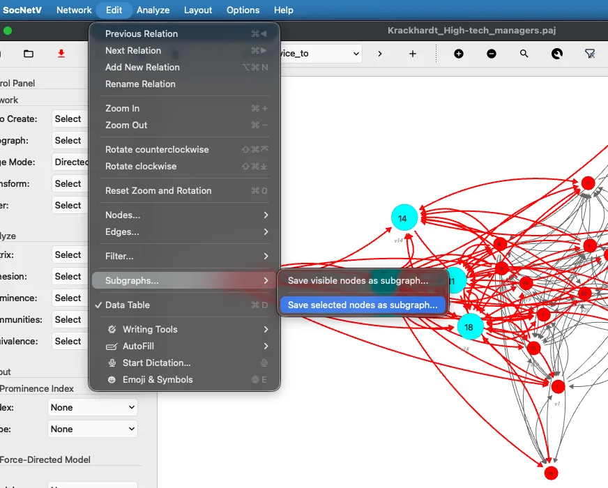
Both dialogs offer all seven supported export formats:
- GraphML — full fidelity; recommended when custom attributes must be preserved.
- Pajek — preserves node labels, colors, shapes, and edge weights; no custom attributes.
- Adjacency Matrix — topology only; active relation only.
- GraphViz DOT — full fidelity for attributes; active relation only; positional roundtrip via
pos=. - UCINET DL — labels and weights; no custom attributes; active relation only.
- Weighted Edge List — labels and weights; active relation only.
- Simple Edge List — labels only; no weights; active relation only.
Structured CSV and JSON (Data Export/Import)
SocNetV v3.5 adds structured CSV and JSON support for exporting and re-importing node and edge attribute data. This is a separate capability from the Adjacency Matrix CSV format, which encodes the graph structure itself.
The feature is accessed through:
- The Data Table dock (
Ctrl+T): Export CSV / Export JSON / Import CSV / Import JSON buttons in each tab. - Network → Export to other…: four menu actions — Nodes as CSV, Edges as CSV, Nodes as JSON, Edges as JSON.
See Data Management for the full workflow.
CSV Format
SocNetV exports and imports RFC 4180 CSV files: a header row followed by one data row per node or edge.
Node CSV example:
#,Label,Size,Color,type,department1,Alice,10,#ff0000,investor,finance2,Bob,7,#0000ff,manager,operations3,Carol,5,#00ff00,analyst,researchEdge CSV example:
Source,Target,Relation,Weight,Label,Color,category,since1,2,friendship,2.5,funds,#333333,partnership,20222,3,friendship,1.0,,#333333,,Column rules on import:
| Column | Behaviour |
|---|---|
# (nodes) / Source + Target (edges) | Used only for row matching; not stored as an attribute |
Label, Size, Color (nodes) | Routed to the proper built-in setters |
Weight, Label, Color (edges) | Routed to the proper built-in setters |
Visible, Shape (nodes) | Read-only — silently skipped |
Relation (edges) | Read-only — silently skipped |
| Any other column | Stored as a custom attribute |
JSON Format
SocNetV exports and imports JSON as a flat array of objects, one object per node or edge. All attribute names become JSON keys.
Node JSON example:
[ { "#": 1, "Label": "Alice", "Size": 10, "Color": "#ff0000", "type": "investor", "department": "finance" }, { "#": 2, "Label": "Bob", "Size": 7, "Color": "#0000ff", "type": "manager", "department": "operations" }]Edge JSON example:
[ { "Source": 1, "Target": 2, "Relation": "friendship", "Weight": 2.5, "Label": "funds", "Color": "#333333", "category": "partnership", "since": "2022" }, { "Source": 2, "Target": 3, "Relation": "friendship", "Weight": 1.0, "Label": "", "Color": "#333333" }]The same column routing rules as CSV apply on import.
Roundtrip Guarantee
Exporting a graph’s node or edge data to CSV or JSON and then re-importing it is a lossless, no-op roundtrip: no duplicate columns are created, no data is lost, and native built-in columns are never accidentally stored as custom attributes.
To persist custom attributes added via import, save the graph in GraphML format (Ctrl+S). See Example 3 in the GraphML section for how those attributes appear in the saved file.